NOMADS_from_nwmTools <- nwmTools::get_nomads_urls(
  output = 'total_water',
  domain = 'atlgulf',
  num = 18,
  version = 'v3.0',
  outdir = ".") %>%
  nwmTools::get_timeseries(
    index_id = c('SCHISM_hgrid_node_x', 'SCHISM_hgrid_node_y'),
    varname  = 'elevation'
  )

NOMADS_from_nwmTools$max <- do.call(pmax, c(NOMADS_from_nwmTools[,3:ncol(NOMADS_from_nwmTools)], list(na.rm=TRUE)))
schism_df_sf <- sf::st_as_sf(NOMADS_from_nwmTools, coords=c("SCHISM_hgrid_node_x","SCHISM_hgrid_node_y")) |>
sf::st_set_crs(sf::st_crs("EPSG:4326"))SCHISM
Executive Summary
Probably best encapsulated by the authors: “SCHISM (Semi-implicit Cross-scale Hydroscience Integrated System Model) is an open-source community-supported modeling system based on unstructured grids, designed for seamless simulation of 3D baroclinic circulation across creek-lake-river-estuary-shelf-ocean scales. It uses a highly efficient and accurate semi-implicit finite-element/finite-volume method with Eulerian-Lagrangian algorithm to solve the Navier-Stokes equations (in hydrostatic form)…”. This model forms the core of OWP’s total water level prediction and has been deployed at scale across a number of domains. (SCHISM Manual at Ccrm-Vims-Edu, n.d.)
Tutorials
Looking at interpolation differences
Pulling the maximum forecast (the easy way)
Pulling the maximum forecast (the hard way)
Sometimes nwmTools might not work as expected, requiring us to perform that data manipulation manually. While this isn’t ideal, I’ve found it to be an occasionally valuable exercise; much like doing math by hand in order to fully grasp the concepts before using a calculator, a foundational understanding of the underlying processes is critical for that next step in explainability. Starting with an understanding of the forecast and releases cycle will help you predict the right timestep to look at, but you can also just try and guess at what you want by clicking around the NOMDAS server. Here we’ll pull in the short range forecast which we know has 18 timesteps, and we’ll brute force our way into the right time with a few handles, and match the format that nwmTools generates because we haven’t already made our lives hard enough.
outpath <- file.path("~/data/output/schism_forecast")
unlink(outpath)
is_quiet <- FALSE

## Get the timestamp for this run
first_valid_timestamp <- format(Sys.time(), tz = "GMT", format = "%Y-%m-%d %H:%M:%S")
first_valid_date <- gsub("-", "",format(Sys.time(), tz = "GMT", format = "%Y-%m-%d"))
first_valid_hour <- format(Sys.time(), tz = "GMT", format = "%H")


# -- Check to make sure I have the right date ---------------------------------------------------------------------------
testurl <- paste0('https://nomads.ncep.noaa.gov/pub/data/nccf/com/nwm/v3.0/nwm.', first_valid_date, '/short_range_coastal_atlgulf')
if (httr::http_error(testurl)) {
  first_valid_date <- gsub("-", "",format(as.Date(first_valid_timestamp, tz = "GMT")-1, format = "%Y-%m-%d"))
}

# -- Guess at the most recent time ---------------------------------------------------------------------------------------
first_valid_hour <- 25
repeat {
  first_valid_hour = first_valid_hour-1
  run_time <- sprintf("%02d", first_valid_hour)
  testurl <- paste0('https://nomads.ncep.noaa.gov/pub/data/nccf/com/nwm/v3.0/nwm.', first_valid_date,'/short_range_coastal_atlgulf/nwm.t', run_time, 'z.short_range_coastal.total_water.f018.atlgulf.nc')
  if(!httr::http_error(testurl)) {
    break
  }
}

first_nomads_timestamp <- strptime(paste0(first_valid_date," ",run_time,':00:00'), format ="%Y%m%d %H:%M:%S",tz = "UTC")
for (i in sprintf("%03d",c(1:18))) {
  # i = sprintf("%03d",c(1:18))[1]
  url <- glue::glue("http://nomads.ncep.noaa.gov/pub/data/nccf/com/nwm/v3.0/nwm.{first_valid_date}/short_range_coastal_atlgulf/nwm.t{run_time}z.short_range_coastal.total_water.f{i}.atlgulf.nc")
  download.file(url, file.path(outpath,"forecast",basename(url),fsep = .Platform$file.sep))
}
all_nc_timesteps <- list.files(file.path(outpath,"forecast",fsep = .Platform$file.sep),pattern = '*.nc$',full.names = TRUE) |> gtools::mixedsort()

nc_file <- ncdf4::nc_open(all_nc_timesteps[1])
x <- ncdf4::ncvar_get(nc_file,"SCHISM_hgrid_node_x")
y <- ncdf4::ncvar_get(nc_file,"SCHISM_hgrid_node_y")
z <- ncdf4::ncvar_get(nc_file,"elevation")

varname <- glue::glue('elevation_{sub("_"," ",ncdf4::ncatt_get(nc_file,0,attname="model_output_valid_time")$value)}')
NOMADS_from_files <- data.frame("SCHISM_hgrid_node_x" = x,
                                "SCHISM_hgrid_node_y" = y,
                                varname = z)
names(NOMADS_from_files)[names(NOMADS_from_files) == "varname"] <- glue::glue('elevation_{sub("_"," ",ncdf4::ncatt_get(nc_file,0,attname="model_output_valid_time")$value)}')
ncdf4::nc_close(nc_file)

j <- length(all_nc_timesteps)
for(i in 2:j) {
  if(!is_quiet) { message(glue::glue("Folding in {i} of {j}")) }
  nc_file <- ncdf4::nc_open(all_nc_timesteps[i])
  NOMADS_from_files$varname <- ncdf4::ncvar_get(nc_file,"elevation")
  names(NOMADS_from_files)[names(NOMADS_from_files) == "varname"] <- glue::glue('elevation_{sub("_"," ",ncdf4::ncatt_get(nc_file,0,attname="model_output_valid_time")$value)}')
  ncdf4::nc_close(nc_file)
}

NOMADS_from_files$max <- do.call(pmax, c(NOMADS_from_files[,3:ncol(NOMADS_from_files)], list(na.rm=TRUE)))

## And the spatial object:
schism_df_sf <- sf::st_as_sf(NOMADS_from_files, coords=c("SCHISM_hgrid_node_x","SCHISM_hgrid_node_y")) |>
  sf::st_set_crs(sf::st_crs("EPSG:4326"))
A few examples of mapping meshes
There are several places to grab mesh elevations but the most authoritative is here:(https://www.nohrsc.noaa.gov/owp_files/nwm/nwm_parameters/README.v3.0.txt). There are a few files we can hunt down to find any differences.
- elev.ic: A .gr3 format file that specifies the initial elevation at each node.
- hgrid.gr3 and hgrid.ll: Horizontal grid file with node centered spatial data and mesh connectivity.
- hgrid.nc: grid file in netcdf format, containing a list of nodes with their locations and elevations along with a list of elements.
- hgrid.vtk: ASCII version of the grid file containing element number, element coordinates, and element original coordinates.
- And NOMADS short range outputs.
Of those, elev.ic seems inappropriate as it represents a “hot” start file since the average node elevation across the database is > 5? hgrid.nc is oddly formatted (as virtually every netcdf file seems to be), but more concretely I’m not seeing an elevation field. Regardless, we can still use the XY as a data point to sanity check. hgrid.vtk is aspatial/unscaled, let’s skip that headache for the time being. That gives us the following:
[1] "Are coordiantes identical?"identical(hgrid.gr3, hgrid.ll):TRUEidentical(hgrid.gr3, hgrid.nc):FALSE| File.testing | Number.of.nodes | Mean.Elevation |
|---|---|---|
| elev.ic | 10537609 | 5.735372 |
| hgrid.gr3 | 10537609 | -4.853219 |
| hgrid.ll | 10537609 | -4.853219 |
| hgrid.nc | 10537609 | NA |
| NOMADS | 10481055 | NA |
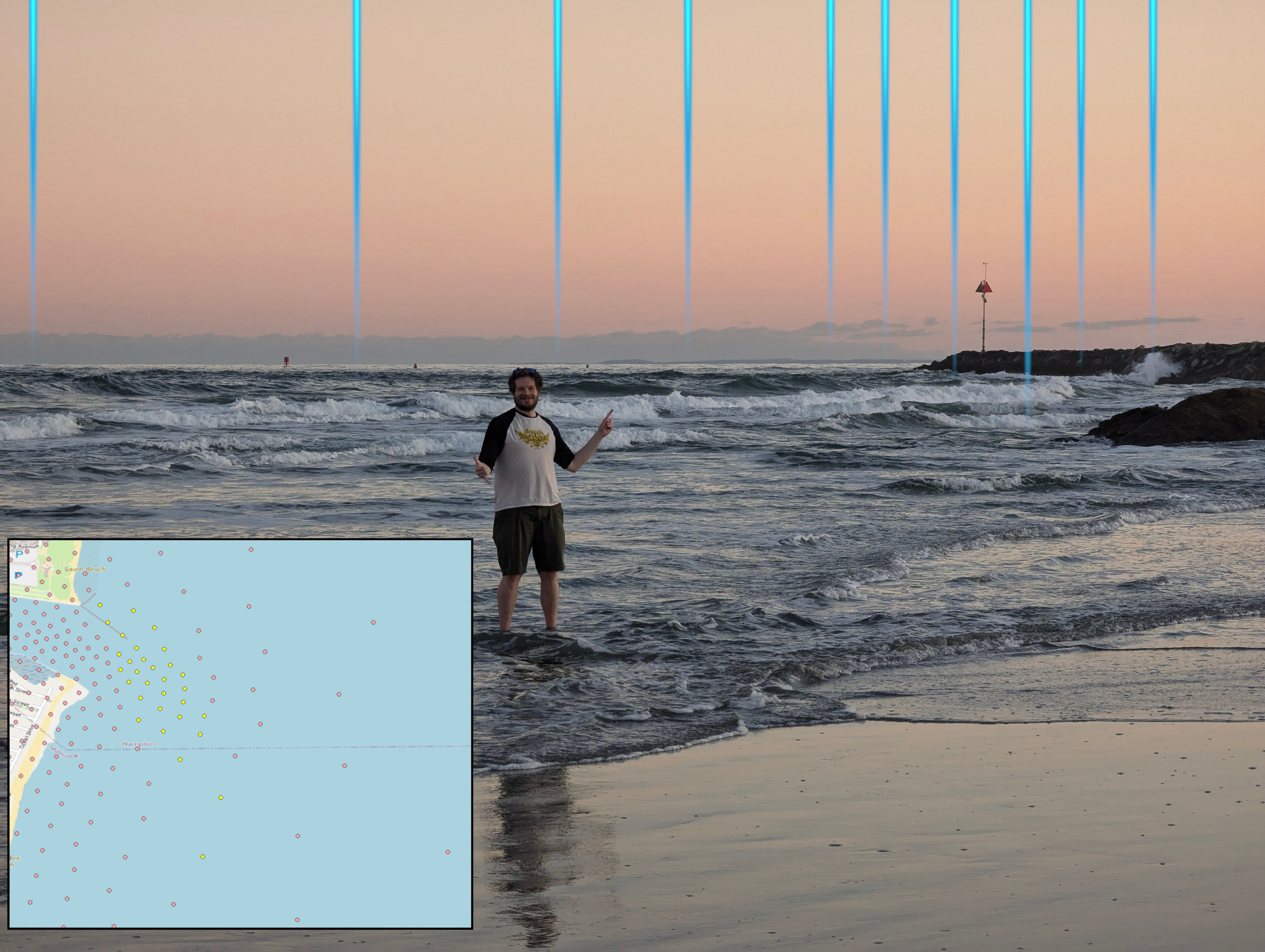
Just to make sure we’re not going insane, let’s take a look at these nodes along the U.S.’s shortest seacoast, New Hampshire!
Loading basemap 'world_imagery' from map service 'esri'...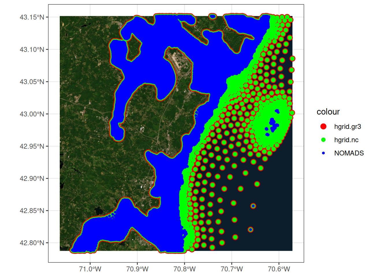
Yup, we’ve lost it.
Mapping a mesh
As a finite element model, SCHISM’s numerical schema is constructed from nodes and the polygons that those nodes define between them. While it’s not typically needed to regenerate the polygons themselves since the model has given us an explicit forecast at the nodes, having access to those shapes is useful. For SCHISM, these are stored in the hgrid.gr3 file, which encodes the node centered spatial data and mesh connectivity as guessable text we can parse out like so:
SCHISM Style Inundation
Reference
Site head: https://ccrm.vims.edu/schismweb/
Online docs: https://schism-dev.github.io/schism/master/index.html
Alternative coastal flooding FIM solutions
NOT comprehensive
The CoastalFlood interface
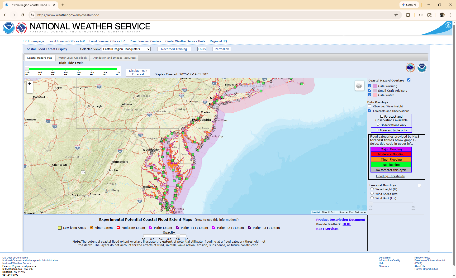
The Eastern Region Headquarters publishes the CoastalFlood service. This service takes the more familiar observation system, normalizes gage datum, and applies a linear interpolation across the various stage impact levels in order to mimic predicted impacts of a sea level forecast to impacts on the landscape. Although a far courser than the SCHISM outputs, this familiarity with both data source and methdology can provide a handy first data point in your decision making process.
Explanations
Coastal FIM
One of the neatest aspects of the total water level forecast is that it’s an explicit prediction of space that can be mapped and evaluated with a “ground truth”. In practice the distinction between modeling surface and mapping surface is lost. To create that surface, we can run a variety of interpolation algorithms. Due to the scale of the SCHISM prediction (continental) and the scale of mapping (building level), an efficient interpolation method is needed in order to meet the needs and concerns of operational flood mapping. Because as we see above, the nodes are close enough that a linear interpolation is beyond sufficient, we’ll precompute depth weights for the mapping surface and deploy a package that performs all the needed steps. See the Coastal-FIM repository for more details.

References
SCHISM Manual at Ccrm-Vims-Edu. n.d. Https://ccrm.vims.edu/schismweb/.