FIM with Jim

Flood Inundation Mapping, or FIM, is the act of mapping what area will be under water for a specified set of conditions. I’ve been fortunate enough to learn from and help River Forecast Centers and the Office of Water Prediction as we undertake the monumental task of generating and operationalizing CONUS scale FIM, pushing the boundaries of Big Data and tackling one of our most pressing wicked problems.
TipOfficial FIM
FIM from the Office of Water Prediction is operational and publicly facing. Check out the landing page at National Water Center Products and the other NOAA resources I’ve pointed to at the top of my junk draw.
FIM with Jim
This “living” page is my home to keep critical background documentation and synthesis of these techniques into what I’ve taken to calling “Geospatial Flood Modeling”, or FrankenFIM.
Common acronyms:
NOAA: National Oceanic and Atmospheric Administration
OWP: Office of Water Prediction
NWM: National Water Model FIM: Flood inundation mapping
HAND: Height Above Nearest Drainage
REM: Relative Elevation Model, occasionally used interchangeably with HAND
SRC: Synthetic Rating Curve
AHG: At a station Hydraulic Geometry
NFIE: National Flood Interoperability Experiment
CFIM: Continental Flood Inundation Mapping Framework out of Oak Ridge National Lab (ORNL), equivalent to…
FIM3: A last major iteration of flood library creation out of NOAA Office of Water Prediction prior to the FIM4 release FIM3 FR: FIM 3 Full-res, an iteration of flood library creation out of NOAA Office of Water Prediction
FIM3-FR/MS: A FIM Full-res/Main stems iteration of flood library creation out of NOAA Office of Water Prediction
FIM4-GMS: FIM Generalized Mainstems - the next iteration of NOAA FIM
RAS2FIM: Wrapper that transforms HEC-RAS 1D BLE models into FIM inputs
Ripple1d: Wrapper that transforms HEC-RAS 1D BLE models into FIM inputs
RRASSLER: A HEC-RAS model accounting system
SCHISM: Semi-implicit Cross-scale Hydroscience Integrated System Model as implemented in and for the National Water model total water level forecast.
FLDPLN: A pixel based geospatial flood model which includes mechanisms that are intended to represent both backfill and spillover flooding.
Find others in my glossary.qmd
Abstract
The computational efficiency of geospatial flood modeling, as opposed to those that solve shallow water flow equations, lend these approaches to real time regional and national scaling. However, the validation of these models remains sparse across both space and time, and no consistent validation metric has been used to quantifiably compare model skill. Furthermore, the pathways from streamflow forecast to flood inundation mapping are an incredibly active area of research. This work provides a high-level overview of several open-source geospatial and low complexity flood inundation mapping techniques, their strengths, costs, and tradeoffs, and the hurdles experienced while performing these tasks.
Background
Flood inundation mapping, or the act of delineating the area under water, is a complex topic that probes deep gaps in our collective knowledge of physical laws governing reality, wrestles us with the technical friction of implementing that theory into operations, and antagonizes us with the with the need for decisive action in situations where every (in)decision has some degree of negative consequence to it. Of these pain points, the technical friction a user experiences when generating a flood inundation map, has recently received a near exponential level-up in difficulty over the last decade with the small renaissance of geospatial flood modeling methods. Geospatial Flood Modeling, as opposed to hydraulic flood modeling, utilizes local, focal, and zonal operations commonly introduced in map algebra curriculum, whereas hydraulic flood modeling typically solves some form of the shallow water flow equations in open channels and can be found in many engineering programs. Although once reserved for large scale analysis, with the trailblazer of the NWM - HAND - Synthetic rating curve demonstrations from the NOAA Office of Water Prediction lead to a dramatic increase in research efforts which formalized and published a number of methods to map a flood, These methods may occasionally emerge from the same organization, but more commonly are created for slightly different use cases, use slightly different terminology, take different pathways towards technical realization, and perhaps most frustratingly, all deploy their drivers in different forms. It is this last point in particular, that each method currently requires it’s own dedicated input stream, that makes intercomparisions between models particularly challenging. To overcome that friction, we propose a framework for interoperable flood mapping efforts which unify these into a set of common input choices which can be easily parsed and passed between methods.
There’s a lot of requisite background knowledge, friction, and occasionally conflicting trade-offs that need to be made between FIM methodology, FIM creation, and FIM operations. FrankenFIM is that bridge (hopefully). To talk about FrankenFIM though, it’s useful to first set the stage for what FIM is and how we use them before we start our interrogation. The first step in that will be to set up some core terminology, most from the field and some from my own making.
As noted, there are a wide variety of FIM libraries and flood modeling algorithms and their origins and lineage are not particularly clear. While not meaningful in terms of implementation or prediction skill, it can be useful to compare and contrast development directions and so to place a few of the key methods I deploy into context, I’ll take a step back and describe the history and lineage of a few of the more popular tools and libraries we use to map flooding.
History of FIM
I’m a poor excuse for a historian, but if I timeline out the different programs and techniques that have been used across the FIM domain, it might look something like this.
What is FIM
FIM, most commonly used as the acronym for Flood Inundation Mapping, is used to refer to activities which comprise the creation of a map which displays the presence or absence of water on the land surface. This is usually represented as a raster of binary values encoding the presence or absence of water, rasters of depth values, or as polygonized representations of contours of those surfaces. One could certainly make the argument that it is not Flood Inundation Mapping but Flood Impact Mapping that is the true end goal, but we’ll avoid that scope creep for now in favor of another, that FIM ought to stand for Flood Inundation Modeling. Many efforts to tease apart the skill and contributions of the techniques end up conflating processes, drivers, and representations, making it impossible to reach a definitive conclusion about what is and is not a “better” approach. Those efforts are further stymied by the different considerations and concerns of the validation metrics and processes deployed that define what that “better” actually is. So, in order to carry out a validation of FIM (A “model bakeoff” in cruder terms), one must construct the FIM libraries using the same model inputs. But what is a FIM Library?
What is a library
I’ve adopted a functional definition for the term FIM Library, which is used to denote a given database. Each of these databases are composed/parsed out in their own particular way, which I refer to as volumes. For example, the CFIM library has volumes which are distributed in a huc6 encoding pattern. The RAS2FIM tool creates libraries whose volumes are distributed with a huc8 and crs pattern. FLDPLN libraries are composed of volumes called segments. The most recent iteration of the OWP HAND approach creates nested volumes generated as huc8’s with many branching libraries. Ripple generates libraries with advanced access patterns that require boundary parameters. A SCHISM library is a singular database, optionally parsed across domains as volumes.
Libraries can also come in different resolutions and different components. Some libraries include rating curves while others are represented soley on elevations or classifications. For a library to be “operational”, it needs to be constructed to a resolution sufficient enough for your objectives, but typically includes many different resolutions and not a handful of predictions. There have been efforts to standardize the data format of a library, the most prominent being the InFRM specifications Wallace (2022). These somewhat arbitrary definitions and terms might at first seem a little unwieldy, but are absolutely critical in order to be able to communicate how we are able to make these methods mesh seamlessly and communicate how the different methods perform.
Other concept nouns you might encounter
Mapping and Modeling
Mapping and Modeling are two distinct tools you might deploy to communicate and/or deploy across your problem solving workflows. Although the for of the outputs often look similar, and many of the tools are the same, the two serve to meet different sets of concerns and represent different views of the same realization. Maintaining the distinctions between these allows us to interoperate between domains more seamlessly, and facilitates a more explainable system.
Precanned? In a box?
While it’s use is not widely standardized, these two concept handles are both used to indicate that the software or results are internally replicable and accessibly formatted for intermediate practitioners. Precanned often shows up alongside FIM results, and indicate that the inundation was calculated or generated with a static parameterization and replicated for the more constrained environment. “In a box” aims to convey that the software and documentation are robust and sufficiently tutorialized so that users who are gaining familiarity in the domain can execute the start of otherwise advanced workflows with minimal configuration and then start their self-guided exploration of the problem space and solutions.
CATFIM?
Following the traditional breakdown of disciplines, inundation maps typically result from a prediction of discharge. However, when indexing impacts it’s standard practice to peg the situation to the stage of the nearest gage. Within the gage network those stages are aggregated to intervals useful for snap decision making with local context. The most common “categories” are a “flood”, “action”, “minor”, “moderate”, “major” clusterings, and are referred to by the stage at the gage of reporting (e.g.: action is at 6 feet). CATFIM is therefore the FIM derived by accessing the libraries using those patterns. This has also been naturally extended to a stage or discharge access pattern, depding on how we query or differ to the linage of the assignment of those catagories.
RPU, VPU, HUC?
Raster Processing Unit (RPU), Vector Processing unit (VPU), and Hydraulic Unit Code (HUC) are all ways in which we can discretize the landscape. The first two in particular are large scale geographic definitions that made computational problems more tractable, particularly when using legacy hydrofabric datasets. They are loosely equivalent to HUC2 units. See my data page for more information.
Normalization
One of the largest but most important factors to accurately capture are changes across the construction of the prediction. Gage networks, although usually static in terms of hardware and setup, are routinely updated with calibrations and modernized to conform to the changing digital standards. Accurately accounting for changes in measurement technique and reporting, particularly as they relate to units, is absolutely critical to get correct. This is further complicated in coastal systems which report values relative to a dynamic datum (sea level) as opposed to the more static gravitational datums of inland systems.
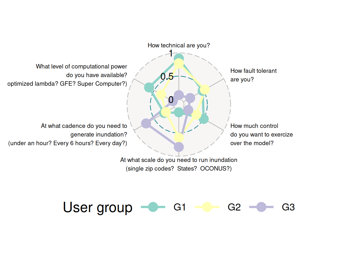
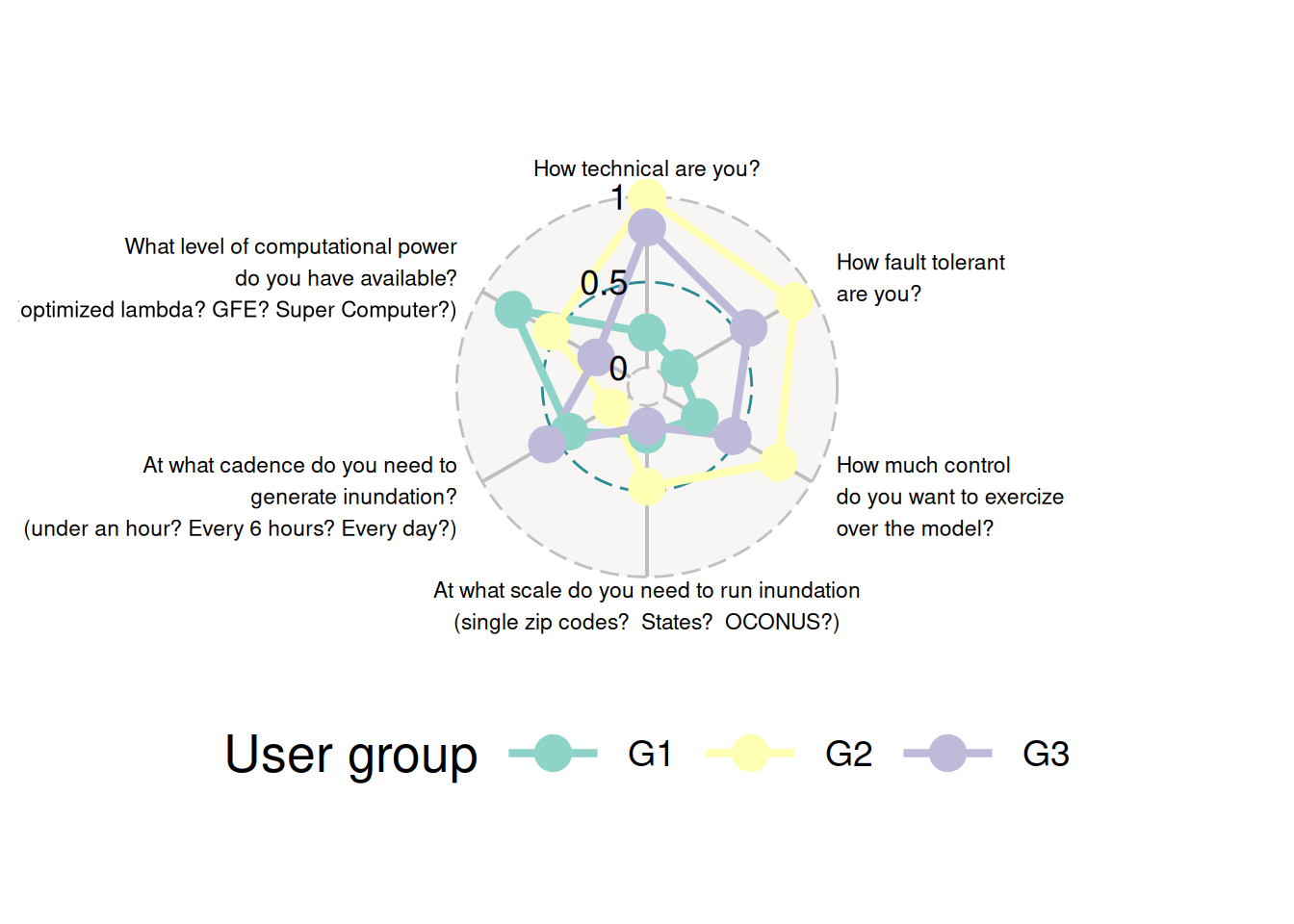
FIM Design Considerations
There are a number of design considerations that one should take into account, and these considerations extend beyond the creation of FIM data to questions like scale and cadence of output generation, fault tolerance, and personally identifiable information (PII) and data security concerns. These considerations need to be addressed before you can start attempting to solve a problem
Methods Overview
There are far too many models and frameworks to enumerate and compare, but to set the stage for the intercomparison, it’s useful to distinguish the different ways a library is constructed.
DEM Subtraction
One of the simplest forms of geospatial FIM is a simplistic cost distance fill, often referred to as a Bathtub fill. These usually require an input DEM, and a gridded set of source cells which serve as the stage of that initial distance operation. Any cell with a value lower than the stage is considered inundated, and anything that is not is considered safe.
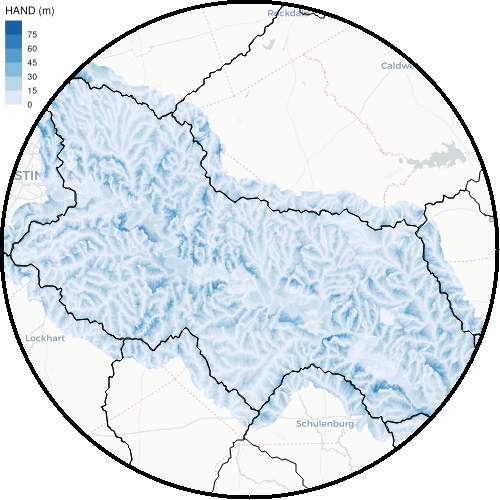
HAND
HAND is a type of relative elevation model that represents the Height Above Nearest Drainage. HAND FIM libraries can come in many forms but the general consensus as it pertains to operational flood mapping is that a viable FIM library contains both the data necessary to translate a discharge into a stage, and a way to place that stage on a map. These most often come in the form of singular rasters of depth assigned a stage, and tied to a river gage as is commonly found in the ahps fim libraries. More recently, that form was altered to accommodate the increased resolution of the river forecast system (manifested in the national water model) by disseminating the rating curves as tables, and geometries as a raster alongside associated depth grids.
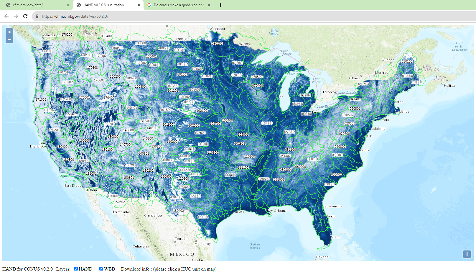
NFIE & CFIM
The first? series of publicly available inundation libraries, this database uses the synthetic rating curve and HAND methodology to transform the output of the National Water Model Channel Routing Outputs to transform a discharge value into a stage and then subtract that stage from the Height Above Nearest Drainage and was first executed on Texas Advanced Computing Center (TACC) resources before further iteration and refinement under the CFIM banner at Oak Ridge National Laboratory.
FIM 3 FR/MS and FIM 4
The evolution of the CFIM workflow from a methodological standpoint, lead by NOAA, resulted in a suite of methodologies which by in large were show to improve the accuracy of the flood map. The first, FIM 3 Full Res (FR) is in essence the CFIM methodology. The second evolution of methodology, FIM 3 Main Stems (MS), addresses inaccuracies at boundaries by refactoring and aggregating the input stream network along a dominant pathway in the watershed. FIM 4, occasionally referenced as Generalized Main Stems (GMS) hallmark improvement was to generalize that refactoring to each branch of the input network. All of these methods share a similar access pattern as well, where the discharge is first converted to stage and then that stage value is used in the HAND subtraction.
Geospatial FIM
FLDPLN
A per pixel representation of libraries which represent both backfill and spillover flooding using geospatial approximations.
Coastal DEM fills
A geospatial approach to coastal inundation modeling, the Eastern Region Headquarters CoastalFlood technique utilizes CO-OPS gages and a linear interpolation of MHHW to create inundation extents directly tied to thresholds with an optional factor of safety (+1-3 feet of elevation). I explore replicating these approaches in this how-to.
Hydraulically derived FIM
USGS and NWS FIM
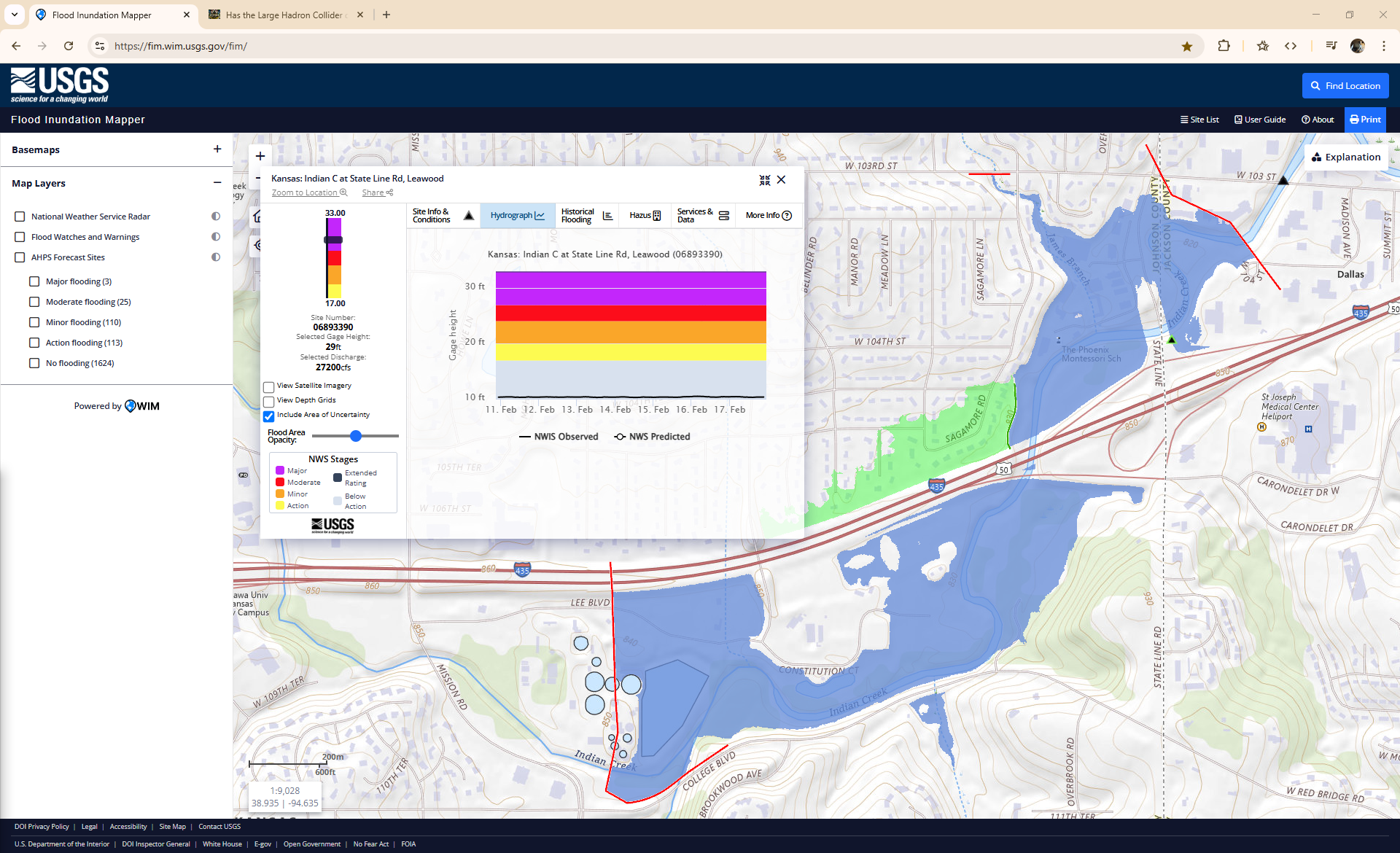
The United States Geologic Survey and the National Water Prediction Service Flood Inundation Maps are a series of stage relative depth maps for each river gage that has a survey. These depth grids are model outputs from contractors who developed hydraulic models and standardized the output. There are two main sources of inundation maps at a federal level. The first is the USGS Flood Inundation Mapping Program (Flood Inundation Mapping (FIM) Program U.S. Geological Survey, n.d.). The second, The National Water Prediction Service Flood Inundation Mapping services through the National Weather Service (NOAA - National Weather Service - Water, n.d.). These two separate databases both reference the same standards document (Dewberry 2011), and are often blended together. I’ve taken to calling this superset of formalized FIM libraries “gage fim”.
RAS2FIM
RAS2FIM automatically formats and runs compliant HEC-RAS 1D models using a densified series of boundary conditions to generate a series of depth grids similar to the AHPS maps while also extracting a representative rating curve for that model. Given the technologic and computational hurdles the software is working around, there are several pain points both before and after the actual execution of the “RAS2FIM” code that make it difficult to elegantly deploy beyond a single domain or for inputs which have not already been pre-canned. To address the first, we introduce RRASSLER, a HEC-RAS model catalog generation and extraction tool to wrestle model data into a standardized and spatially accessible format. To address the latter, RAS2REM was created, which reformats RAS2FIM outputs into a geospatially accessible flood libraries.
SCHISM
SCHISM (Semi-implicit Cross-scale Hydroscience Integrated System Model) is an unstructured mesh which forecasts a water surface elevation for a set of boundary conditions across large scales. Past iterations of the modal have nodes which can be closer than 5 meters or as far away as 2000 meters. The current iteration has more than 10 million nodes across the Atlantic and Gulf domains.
Other Coastal inundation
Other Coastal Models
Outside of the ERH/OWP Coastal CATFIM efforts, most coastal modeling efforts lean heavily into the numerical representations and so are most appropriate. See National Operational Coastal Modeling Program (NOCMP) for the various models and domains that NOS produces.
FLDPLN and Operational Flood Inundation Mapping in Kansas
Flood inundation maps are needed for emergency response and planning. We present an operational flood inundation mapping (FIM) system which covers the eastern two-thirds of the State of Kansas which and provides both current and forecasted flood inundation depth maps using observed gage stages. The system is based on the low-complexity FLDPLN FIM model which considers both backfill and spillover mechanisms to and generates flood inundation relations between stream channel cells and flood plain cells. We present the assessment on the FLDPLN model and compare it with the Height Above Nearest Drainage (HAND) FIM model used for nation-wide operational flood inundation mapping at the Office of Water Prediction (OWP) National Water Center. The mapping component of the system organizes the flood inundation relations as tiles in space, and takes the advantage of parallel computing to speed up inundation mapping. In addition, the system provides an example of computing maps using spatial relationships, which is a new geospatial data analysis framework currently under development.
Healing a map/model surface
One of the goals of a FIMap is to communicate the area inundated across the terrain. Depending on how familiar you are with reading a FIMap or you’re reading the map for a particular purpose, you may find yourself wondering if a particular asset is impacted by the flood. One of the most common ways we want to make a map more reflective of the conditions and uses is to place bridge representations back into the model surface in order to represent whether or not the bridge was expected to be impacted.
References
Dewberry. 2011. Guidelines for the Development of Advanced Hydrologic Prediction Service Flood Inundation Mapping. NOAA.
Flood Inundation Mapping (FIM) Program U.S. Geological Survey. n.d. Https://www.usgs.gov/mission-areas/water-resources/science/flood-inundation-mapping-fim-program.
NOAA - National Weather Service - Water. n.d. Https://water.weather.gov/ahps/inundation.php.
Wallace, David S. 2022. Flood Decision Support Toolbox Executive Summary and Submittal Guidance.