Accuracy
When communicating the results of an analysis, one of the first questions anyone will ask you is if you calibrated/validated your model. Often, this is a loaded question for a number of reasons, but one of the most addressable ones is to provide them the accuracy metric of your choice. While not always the case, this generally involves comparing two rasters, a reference and a ground truth to create what is known as a “confusion matrix”. This combination of values can be mathematically reduced to a single value, and that singular number is all that’s usually reported.
This of course can get the box checked at the end of the day, but leaves quite a lot of room for improvement. One of the “easiest” ways to improve on this baseline though, is to continue to perform that accuracy assessment at regular intervals. The single marker in that time series may not mean much in isolation, but when you can show steady or incremental improvements in that metric over time, that lends confidence to the underlying process representations you are applying to your model.
The other game to play here is of course the “which metric do you choose?” game. Much like an extremely accessible form of p-hacking, They take catchment aggregated p-bias and take that as the room temperature measurement. “If water model versions are making improvements in each iteration that is seen as the sign that these efforts are improving. That is misleading not only because they’ve hinged that outcome on a single metric with no spatial significance, but also because the calibration and validation data is treated as a monolitic and stable set of observations instead of a living collection of data points which have a seasonality and even event based alternatives.
| Truth Positive |
True Positive (A) |
False Negative (B) |
Null Positive (E) |
| Truth Negative |
False Positive (C) |
True Negative (D) |
Null Negative (F) |
| Truth Null |
Unverifiable Hit (G) |
Unverifiable Rejection (H) |
|
Common metrics
The hydrologic and hydraulic communities have a select number of accuracy metrics and traditional workflows that they reach to when they try to quantify the skill or performance of a model.
| Bias |
Continuous |
Long term average error (dry/wet) - also forcings |
| RMSE / RSR Nash-sutcliffe |
Cont |
A set of standard variance estimators, sometimes applied to long(Q) to de-emphasize extremes |
| Correlation |
Cont |
Linear correlation coefficient (Pearson’s r) |
| Kling-Gupta efficiency |
Cont |
Rational decomposition of error components (linear correlation, variability bias, and mean bias) |
| Peak discharge |
event |
Ability of model to predict Qp for events |
| Stormflow error |
event |
Ability of model to predict Rp for events |
| Conditional |
event |
Occurrence of an event (TP,FP,TN,FN) |
| Peak timing |
event |
Ability of model to predict Tp for events |
| Hydrologic signature |
mixed |
Other information content in streamflow signal |
Acc
Hydrologists lean to several common metrics but one of the most common is nash-sutcliffe.
Carson plots provide a rich overview of comparisons by tracking 3 of the 4 confusion matrix values alongside an aggregate metric of the designers choice.
SNOTEL is a series of stations set up primarily along the Rockies that include a series of advanced sensors to measure precipitation. The king of the show is the snow pillow, which measures the weight of snow on top of it, and can be used to calculate the snow water equivalent.
Metrics matter
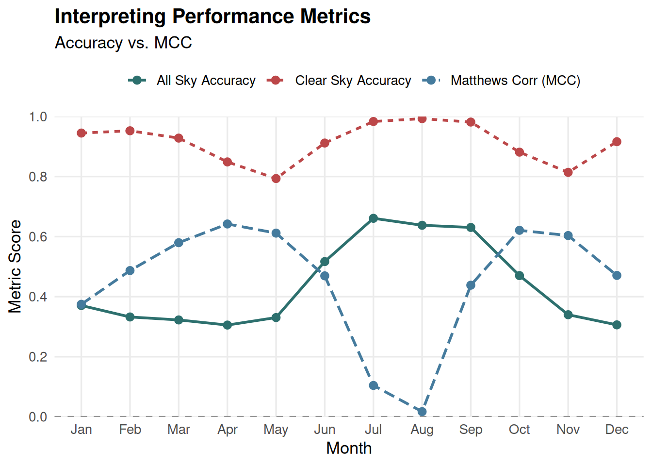
I don’t have many pet peeves but one of them is listening to a conversation that poorly deploys or interprets accuracy metrics. Much of that frustration comes because those conversation tend to poorly wield these otherwise powerful aggregate statistics in a way that might be inappropriate, or that the “blame” for the poor performance is pinned to a misunderstanding of how variations in the confusion matrix do or do not impact the resulting calculation. One of the simplest ways I can try and describe this is along the lines of a paper on snow cover accuracy I wrote many moons ago. In this, we are comparing accuracy of two measurements, one, a SNOTEL snow pillow and two, a MODIS snow cover pixel. Taking the data from Table 3 of [@collComprehensiveAccuracyAssessment2018],
| Month |
1 |
2 |
3 |
4 |
5 |
6 |
7 |
8 |
9 |
10 |
11 |
12 |
| A |
99,134 |
80,492 |
83,064 |
63,886 |
30,313 |
5,538 |
171 |
8 |
1,237 |
18,951 |
64,085 |
79,714 |
| B |
5,473 |
3,779 |
6,284 |
13,287 |
21,423 |
11,733 |
2,268 |
140 |
1,033 |
11,432 |
16,762 |
6,627 |
| C |
397 |
330 |
502 |
1,004 |
1,937 |
1,441 |
790 |
1,151 |
2,136 |
5,737 |
3,620 |
985 |
| D |
1,355 |
1,655 |
4,407 |
16,302 |
59,356 |
130,360 |
179,941 |
174,369 |
166,161 |
108,457 |
25,111 |
3,292 |
| E |
163,031 |
159,109 |
172,667 |
152,530 |
98,668 |
25,731 |
1,586 |
172 |
3,415 |
44,574 |
125,803 |
175,798 |
| F |
1,839 |
1,827 |
4,366 |
15,548 |
59,702 |
88,136 |
87,754 |
97,594 |
91,506 |
81,879 |
27,115 |
4,859 |
| AC |
0.945 |
0.952 |
0.928 |
0.849 |
0.793 |
0.912 |
0.983 |
0.993 |
0.981 |
0.881 |
0.814 |
0.916 |
| AA |
0.370 |
0.332 |
0.322 |
0.305 |
0.330 |
0.517 |
0.661 |
0.638 |
0.630 |
0.470 |
0.340 |
0.306 |
| MCC |
0.374 |
0.487 |
0.580 |
0.642 |
0.612 |
0.469 |
0.104 |
0.017 |
0.438 |
0.621 |
0.604 |
0.471 |
| A AB |
0.948 |
0.955 |
0.930 |
0.828 |
0.586 |
0.321 |
0.070 |
0.054 |
0.545 |
0.624 |
0.793 |
0.923 |
| D DC |
0.773 |
0.834 |
0.898 |
0.942 |
0.968 |
0.989 |
0.996 |
0.993 |
0.987 |
0.950 |
0.874 |
0.770 |
A note on accuracy in the aggregate
@klotzTechnicalNoteDivide2024
accuracy in the context of snow cover presence
See the full paper in remote sensing: Comprehensive accuracy assessment of MODIS daily snow cover products and gap filling methods
One of my earliest forays into accuracy reporting was comparing how well the fractional snow cover valve from MODIS compared with SNOTEL sites. As a new student to the discipline, I had quite a few questions about how best to approach reporting model behavior, and was interested in describing the way we study accuracy.
This study was quite novel for it’s time due to the sweeping scale that the use of Google Earth Engine provided and the cutting edge nature of the factional snow cover band in the then new MODIS V6 product contained. When I have the time and direction to push back into this space, I feel a site specific exploration of these properties would be insightful.