Precipitation

Executive Summary

Water flows down-gradient, and in the case of precipitation initiated by phase changes and atmospheric cooling it typically flows towards the surface of the earth as gravitational potential overcomes aerodynamic drag (terminal velocity). When it’s frozen, we call that snow.

References

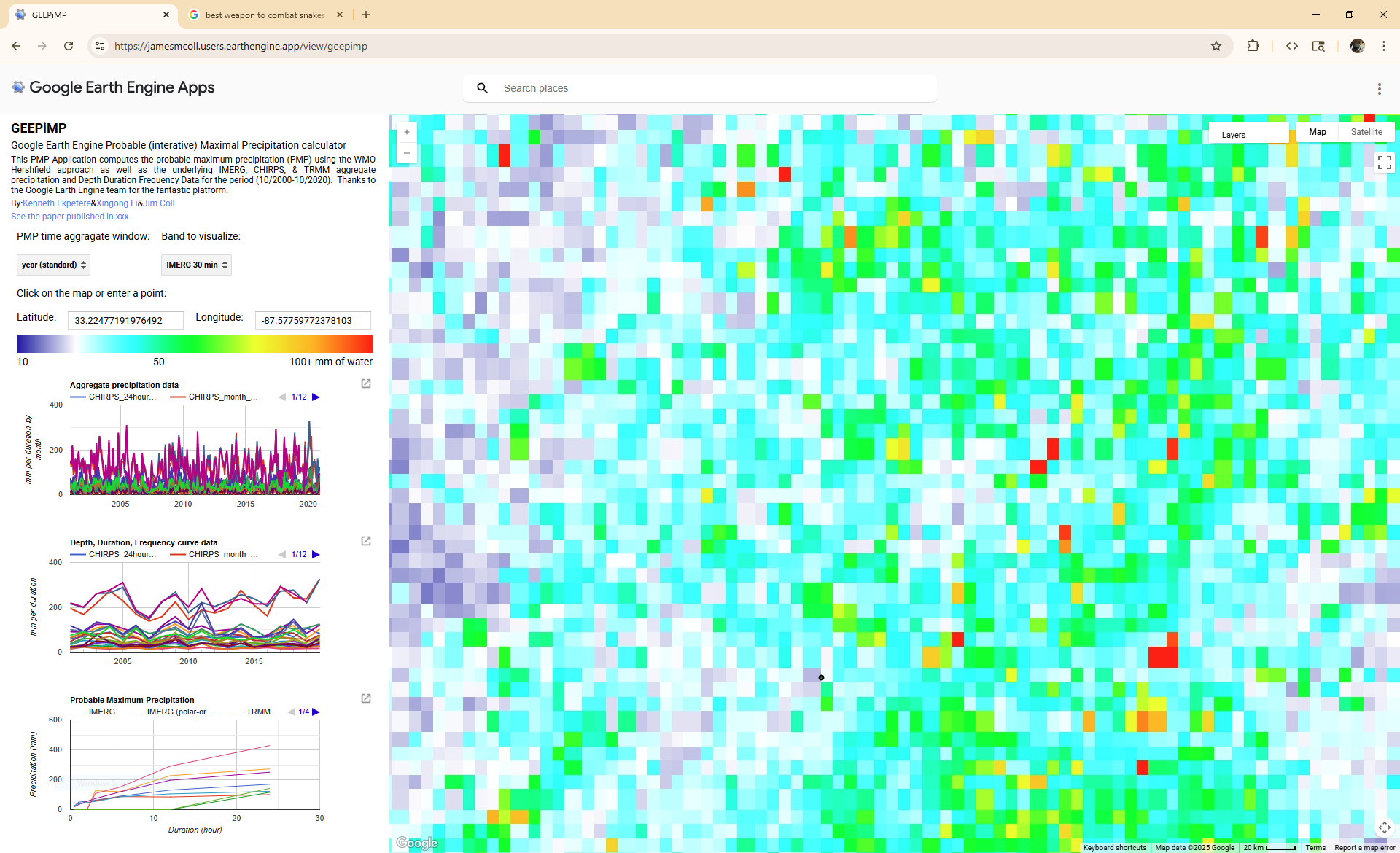
Use the interactive application to rapidly pull PMP values for a point.

Tutorials

Explanations:

See a verbose explainer following the method used to calculate Probable Maximum Precipitation.
How we transform Flood frequency analysis.

Relates

What would be the other alternatives to get a precipitation return period / intensity