Simple feature collection with 2111 features and 11 fields
Geometry type: LINESTRING
Dimension:     XY
Bounding box:  xmin: -71.84246 ymin: 41.1535 xmax: -71.12936 ymax: 42.01646
Geodetic CRS:  WGS 84
First 10 features:
     osm_id                          name       highway waterway aerialway
1   5386504    East Providence Expressway      motorway     <NA>      <NA>
2   9631965                 School Street      tertiary     <NA>      <NA>
3   9695083             Washington Street       primary     <NA>      <NA>
4  17165773              Boom Bridge Road   residential     <NA>      <NA>
5  19347944                          <NA> motorway_link     <NA>      <NA>
6  19348740     Gladys Carr Bolhouse Road  unclassified     <NA>      <NA>
7  19349618           Weenachasett Bridge    pedestrian     <NA>      <NA>
8  19352492                          <NA> motorway_link     <NA>      <NA>
9  19353027            South County Trail       primary     <NA>      <NA>
10 19353594 Woonsocket Industrial Highway      motorway     <NA>      <NA>
   barrier man_made railway bridge z_order
1     <NA>     <NA>    <NA>    yes      29
2     <NA>     <NA>    <NA>    yes      24
3     <NA>     <NA>    <NA>    yes      27
4     <NA>     <NA>    <NA>    yes      23
5     <NA>     <NA>    <NA>    yes      29
6     <NA>     <NA>    <NA>    yes      23
7     <NA>     <NA>    <NA>    yes      20
8     <NA>     <NA>    <NA>    yes      29
9     <NA>     <NA>    <NA>    yes      27
10    <NA>     <NA>    <NA>    yes      29
                                                                                                                                                                                                                                                                                                                                                                                                                                                                 other_tags
1  "bicycle"=>"no","check_date"=>"2025-07-02","foot"=>"no","hgv"=>"designated","hgv:national_network"=>"yes","horse"=>"no","lanes"=>"3","layer"=>"1","maxheight"=>"13'5\\"","maxspeed"=>"40 mph","oneway"=>"yes","ref"=>"I 195;US 1A;US 6","source:hgv:national_network"=>"https://www.ecfr.gov/current/title-23/chapter-I/subchapter-G/part-658;https://hepgis-usdot.hub.arcgis.com/apps/usdot::national-network-conventional-combination-trucks-map","surface"=>"asphalt"
2                                                                                                                                                                                                                                                               "attribution"=>"Office of Geographic and Environmental Information (MassGIS)","condition"=>"fair","hgv"=>"yes","lanes"=>"2","layer"=>"1","massgis:way_id"=>"200497","source:hgv"=>"MassGIS","width"=>"12.2"
3                                                                                                                                              "attribution"=>"Office of Geographic and Environmental Information (MassGIS)","condition"=>"fair","hgv"=>"yes","lanes"=>"4","layer"=>"1","massgis:way_id"=>"191505","maxspeed"=>"40 mph","ref"=>"US 1","sidewalk:both"=>"separate","source:hgv"=>"MassGIS","source:maxspeed"=>"massgis","surface"=>"asphalt","width"=>"19.8"
4                                                                                                                                                                                                                                                                                                                                                          "layer"=>"1","tiger:cfcc"=>"A41","tiger:name_base"=>"Boom Bridge","tiger:name_type"=>"Rd","tiger:reviewed"=>"no"
5                                                                                                                                                                                                                                                                                                                                                                             "layer"=>"1","oneway"=>"yes","surface"=>"asphalt","tiger:cfcc"=>"A63","tiger:reviewed"=>"yes"
6                                                                                                                                                                                                                                                                                                                                                                                                               "layer"=>"1","tiger:cfcc"=>"A41","tiger:reviewed"=>"aerial"
7                                                                                                                                                                                                                                                                                                                                                                                                 "access"=>"private","layer"=>"1","surface"=>"asphalt","tiger:cfcc"=>"A49"
8                                                                                                                                                                                                                                                                                                                        "destination"=>"Atwells Avenue","junction:ref"=>"37A","lanes"=>"1","layer"=>"1","maxspeed:advisory"=>"30 mph","oneway"=>"yes","surface"=>"asphalt"
9   "hgv"=>"designated","lanes"=>"2","layer"=>"1","maxspeed"=>"35 mph","oneway"=>"yes","ref"=>"RI 2","source:hgv"=>"https://www.arcgis.com/apps/mapviewer/index.html?webmap=090921ccfeab455e8da224ba9b75d213;https://gisstage.dot.ri.gov/Approved53FtSemiTrailerRoutes.pdf","surface"=>"asphalt","tiger:cfcc"=>"A25","tiger:name_base"=>"County","tiger:name_base_1"=>"State Highway 2","tiger:name_direction_prefix"=>"S","tiger:name_type"=>"Trl","tiger:reviewed"=>"yes"
10                                                                                                                                                                                                 "hgv"=>"designated","lanes"=>"2","layer"=>"1","oneway"=>"yes","ref"=>"RI 99","source:hgv"=>"https://www.arcgis.com/apps/mapviewer/index.html?webmap=090921ccfeab455e8da224ba9b75d213;https://gisstage.dot.ri.gov/Approved53FtSemiTrailerRoutes.pdf","surface"=>"asphalt"
                         geometry
1  LINESTRING (-71.38436 41.81...
2  LINESTRING (-71.32944 41.78...
3  LINESTRING (-71.37107 41.89...
4  LINESTRING (-71.82341 41.41...
5  LINESTRING (-71.48019 41.72...
6  LINESTRING (-71.32293 41.49...
7  LINESTRING (-71.32458 41.51...
8  LINESTRING (-71.41898 41.82...
9  LINESTRING (-71.49195 41.61...
10 LINESTRING (-71.48499 41.95...OpenStreetMaps
Infrastructure
Operational
An open source community effort to digitize the transportation network of the world, facilitated through the OpenStreetMap Foundation.
Back to Data Sources
Open Street Maps
The OpenStreetMap (OSM), and in particular the dataset underlying the map, is a collaborative effort to create a free and editable map of the world. Its efforts aim to capture the geographic position and associated metadata of locations and assets like buildings and roads contributed by volunteers.
Novel or otherwise noteworthy aspects of this dataset include its open nature and reuse license (anyone can access and use the data under the Open Data Commons Open Database License (ODbL)). It also has global coverage and covers a number of different asset types, as opposed to something like OpenAddresses which is more US-centric and oriented towards address points.
Data Structure
To effectively use OSM in R, it helps to understand the three core elements:
- Nodes: Points in space (coordinates). Used for POIs or defining the shape of lines.
- Ways: Ordered lists of nodes. Open ways are lines (roads, streams); closed ways are polygons (buildings, parks).
- Relations: Groups of nodes, ways, or other relations. Used for complex logical connections (e.g., a bus route consisting of many road segments).
The common OSM Ecosystem
While there are many tools to access OSM, the R ecosystem provides several targeted packages:
| Package | Best For |
|---|---|
| osmextract | High Volume. Downloading and reading large .pbf files (e.g., whole states or countries). It uses GDAL/SQL logic to keep memory usage low. |
| osmdata | Precision. Querying the Overpass API for small, specific datasets (e.g., “all cafes in downtown Seattle”). |
| OSMnx | Network Analysis. A Python library, but often used alongside R via reticulate for topology cleaning and street network analysis. |
HOW-TO: Extracting Bridge Lines at Scale
Extracting infrastructure (like bridges) changes drastically depending on your spatial scale. Loading a state is easy; loading the Contiguous United States (CONUS) will crash most R sessions if not handled via out-of-memory databases.
Below are the patterns for State, VPU (Regional), and CONUS scale extractions.
State Scale
At the state scale, osmextract::oe_get() is your best tool. It will download the Geofabrik .pbf for the state, translate it to a GeoPackage, and load it into RAM as an sf object. We use an SQL query to filter for bridges during the translation to save memory.
VPU Scale
If you are working with VPUs or domains that cross state lines, you can use a spatial boundary to clip the data during extraction.
path_to_data <- "~/data/raw"
is_verbose <- FALSE

path_to_gdb <- file.path(path_to_data,"WBD_National_GDB/WBD_National_GDB.gdb",fsep = .Platform$file.sep)
huc2 <- sf::st_read(path_to_gdb,layer = 'WBDHU2',quiet=!is_verbose)

vpu_polygon <- huc2[huc2$huc2 == '01',]

# Use oe_vectortranslate with a spatial boundary clip
# vpu_bridges_path <- osmextract::oe_vectortranslate(
#   file_path = "~/data/raw/OSM/north-america-latest.osm.pbf",
#   layer = "lines",
#   extra_tags = c("bridge"),
#   vectortranslate_options = c("-where", "bridge IS NOT NULL AND bridge != 'no'"),
#   boundary = vpu_polygon,
#   boundary_type = "spat", # Uses spatial intersection
#   quiet = FALSE
# )

# This made a geopackage
vpu_bridges_path <- file.path(path_to_data,"OSM","north-america-latest.gpkg")

vpu_bridges <- sf::st_read(vpu_bridges_path)
Reading layer `lines' from data source
`/home/rstudio/data/raw/OSM/north-america-latest.gpkg' using driver `GPKG'
Simple feature collection with 992378 features and 11 fields
Geometry type: LINESTRING
Dimension: XY
Bounding box: xmin: -179.4675 ymin: 14.553 xmax: 175.8839 ymax: 82.48983
Geodetic CRS: WGS 84vpu_bridgesSimple feature collection with 992378 features and 11 fields
Geometry type: LINESTRING
Dimension: XY
Bounding box: xmin: -179.4675 ymin: 14.553 xmax: 175.8839 ymax: 82.48983
Geodetic CRS: WGS 84
First 10 features:
osm_id name highway waterway aerialway barrier
1 368044 Chester Road primary <NA> <NA> <NA>
2 3074293 Fountain Street North secondary <NA> <NA> <NA>
3 3129874 Pasadena Avenue secondary <NA> <NA> <NA>
4 3144039 Avenue 19 tertiary <NA> <NA> <NA>
5 3144312 Los Feliz Boulevard primary <NA> <NA> <NA>
6 3474126 Highway 102 motorway <NA> <NA> <NA>
7 3696127 <NA> motorway_link <NA> <NA> <NA>
8 3696128 Don Valley Parkway motorway <NA> <NA> <NA>
9 3831351 Garden Grove Freeway motorway <NA> <NA> <NA>
10 3886657 <NA> motorway_link <NA> <NA> <NA>
man_made railway bridge z_order
1 <NA> <NA> yes 27
2 <NA> <NA> yes 26
3 <NA> <NA> yes 26
4 <NA> <NA> yes 24
5 <NA> <NA> yes 27
6 <NA> <NA> yes 29
7 <NA> <NA> yes 29
8 <NA> <NA> yes 29
9 <NA> <NA> yes 29
10 <NA> <NA> yes 29
other_tags
1 "hgv"=>"designated","layer"=>"1","maxspeed"=>"40 mph","old_ref_legislative"=>"225","ref"=>"PA 320","source:hgv"=>"https://www.dot.state.pa.us/public/pubsforms/Publications/TruckersMap.pdf"
2 "cycleway:both"=>"lane","layer"=>"1","maxspeed"=>"50","ref"=>"RR 17"
3 "lanes"=>"4","layer"=>"1","maxspeed"=>"35 mph","maxspeed:conditional"=>"25 mph @ children_present","old_ref"=>"US 66;US 99","placement:backward"=>"left_of:1","source:maxspeed"=>"survey;image","source_ref"=>"AM909_DSCV1642","source_ref:maxspeed"=>"AM909_DSCV1645"
4 "cycleway"=>"track","layer"=>"1","old_ref"=>"US 99","oneway"=>"yes"
5 "bridge:name"=>"Los Feliz Blvd","bridge_ref"=>"5/LA/53-1070","lanes"=>"3","layer"=>"1","milepost:county"=>"24.33","oneway"=>"yes","placement"=>"right_of:2","source:bridge"=>"usgs_imagery;survey;image;CDOT","source_ref:bridge"=>"AM909_DSCV3547","turn:lanes"=>"||merge_to_left"
6 "NHS"=>"yes","alt_name"=>"Veterans Memorial Highway","destination"=>"Halifax","destination:symbol"=>"airport","direction"=>"S","lanes"=>"3","layer"=>"1","maxheight"=>"4.1","maxspeed"=>"100","official_name"=>"Highway 102","oneway"=>"yes","ref"=>"NS 102","surface"=>"asphalt"
7 "destination"=>"Downtown","destination:ref"=>"DVP South","destination:street"=>"Don Valley Parkway South","lanes"=>"2","layer"=>"1","maxspeed"=>"100","oneway"=>"yes","surface"=>"asphalt"
8 "lanes"=>"3","layer"=>"1","lit"=>"yes","maxspeed"=>"100","noref"=>"yes","oneway"=>"yes","surface"=>"asphalt"
9 "bicycle"=>"no","hgv"=>"designated","hgv:national_network"=>"terminal_access","lanes"=>"2","layer"=>"1","maxspeed"=>"65 mph","maxspeed:hgv"=>"55 mph","maxspeed:trailer"=>"55 mph","oneway"=>"yes","ref"=>"CA 22","source:hgv:national_network"=>"Caltrans http://www.dot.ca.gov/hq/traffops/trucks/truckmap/","surface"=>"concrete"
10 "bicycle"=>"no","destination"=>"Colorado Boulevard;Orange Grove Boulevard","junction:ref"=>"13A","lanes"=>"1","layer"=>"1","lit"=>"yes","old_ref"=>"SR 248","old_ref:legislative"=>"161","oneway"=>"yes"
geometry
1 LINESTRING (-75.36147 39.87...
2 LINESTRING (-80.37125 43.40...
3 LINESTRING (-118.2196 34.07...
4 LINESTRING (-118.2259 34.07...
5 LINESTRING (-118.2711 34.12...
6 LINESTRING (-63.31599 45.36...
7 LINESTRING (-79.33863 43.76...
8 LINESTRING (-79.33888 43.76...
9 LINESTRING (-118.0842 33.77...
10 LINESTRING (-118.1653 34.14...# Inspection & Visualization
path_to_basedata <- "~/Dropbox/root/database/hosted"
states <- sf::st_read(file.path(path_to_basedata,"admin/tiger/TIGER2022/STATE/tl_2022_us_state/tl_2022_us_state.fgb",fsep = .Platform$file.sep),
query = glue::glue("SELECT * FROM tl_2022_us_state WHERE GEOID < '57%' AND GEOID NOT LIKE '02%' AND GEOID NOT LIKE '15%'"),
quiet=!is_verbose)
states_filter <- sf::st_transform(states, sf::st_crs(vpu_bridges))
states_5070 <- sf::st_transform(states, 5070)
bridges_filtered <- vpu_bridges |> sf::st_filter(states_filter) |> sf::st_transform(5070)
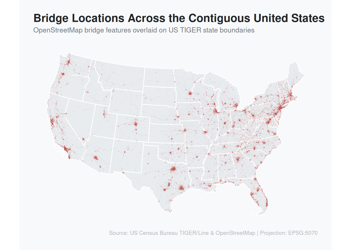
# 2. Build map
ggplot2::ggplot() +
# Base state polygons
ggplot2::geom_sf(data = states_5070, fill = "#e8ecef", color = "#ffffff", linewidth = 0.5) +
# Bridges layer (warm coral overlay)
ggplot2::geom_sf(data = bridges_filtered, color = "#d9534f", alpha = 0.5, linewidth = 0.25) +
# Coordinate system & clean crop
ggplot2::coord_sf(crs = sf::st_crs(5070), datum = NA) +
ggplot2::labs(
title = "Bridge Locations Across the Contiguous United States",
subtitle = "OpenStreetMap bridge features overlaid on US TIGER state boundaries",
caption = "Source: US Census Bureau TIGER/Line & OpenStreetMap | Projection: EPSG:5070"
) +
ggplot2::theme_void() +
ggplot2::theme(
plot.background = ggplot2::element_rect(fill = "#f8f9fa", color = NA),
panel.background = ggplot2::element_rect(fill = "#f8f9fa", color = NA),
plot.title = ggplot2::element_text(color = "#212529", size = 16, face = "bold", hjust = 0, margin = ggplot2::margin(b = 4)),
plot.subtitle = ggplot2::element_text(color = "#6c757d", size = 10, hjust = 0, margin = ggplot2::margin(b = 15)),
plot.caption = ggplot2::element_text(color = "#adb5bd", size = 8, hjust = 1, margin = ggplot2::margin(t = 10)),
plot.margin = ggplot2::margin(t = 20, r = 20, b = 20, l = 20)
)
CONUS Scale Extraction (DuckDB & SpatiaLite)
When processing the entire US (us-latest.osm.pbf), do not use oe_get() to load the result into R memory. Instead, translate the PBF into a SpatiaLite or GeoPackage database, and use DuckDB to query it out-of-memory.
Step A: Translate .osm.pbf to a spatially indexed GeoPackage
This step can take 15–30 minutes for CONUS, but only needs to be run once.
# Translate the raw US PBF to a GeoPackage, extracting ONLY bridge lines
conus_bridge_gpkg <- osmextract::oe_vectortranslate(
  file_path = "~/data/raw/OSM/north-america-latest.osm.pbf",
  layer = "lines",
  extra_tags = c("bridge", "highway", "waterway"),
  query = "SELECT * FROM lines WHERE bridge IS NOT NULL AND bridge != 'no'",
  quiet = FALSE
)
Step B: Query with DuckDB: DuckDB’s spatial extension is incredible for querying massive OSM files directly from disk.
library(duckdb)
library(DBI)
library(sf)

# Connect to an in-memory DuckDB instance
con <- DBI::dbConnect(duckdb::duckdb())

# Install and load the spatial extension
dbExecute(con, "INSTALL spatial;")
dbExecute(con, "LOAD spatial;")

# Define the query using ST_Read to access the GeoPackage we just built
# We cast the geometry to WKB (Well-Known Binary) so sf can parse it natively
query <- "
  SELECT
    osm_id,
    highway,
    bridge,
    ST_AsWKB(geom) as geometry
  FROM ST_Read('~/data/raw/OSM/us-latest.gpkg')
  WHERE highway = 'motorway' -- Example: further filtering to only major highway bridges
"

# Execute query and pull into R as a standard data.frame
result_df <- dbGetQuery(con, query)

# Convert the WKB column to an active sf geometry column
conus_major_bridges <- sf::st_as_sf(result_df, wkb = "geometry", crs = 4326)

# Always disconnect
DBI::dbDisconnect(con, shutdown = TRUE)

conus_major_bridges
mapview::mapview(conus_major_bridges, zcol = "bridge", legend = TRUE)
Alternative: Transform to SpatiaLite via Command Line
If you prefer operating outside of the R osmextract wrappers for massive files, you can invoke GDAL’s ogr2ogr directly via a system call to create a highly optimized SpatiaLite database.
library(duckdb)
library(DBI)

in_pbf <- "~/data/raw/OSM/north-america-latest.osm.pbf"
out_dbase <- "~/data/raw/OSM/osm_tests.sqlite"

# Note: Requires GDAL to be installed on your system
full_command <- paste(
  "ogr2ogr -f SQLite",
  shQuote(out_dbase),
  shQuote(in_pbf),
  "-dsco SPATIALITE=YES",
  "-lco SPATIAL_INDEX=YES",
  "-gt 65536",
  "--config OSM_MAX_TMPFILE_SIZE 4096",
  "-oo USE_CUSTOM_INDEXING=YES",
  "-oo COMPRESS_NODES=YES"
)

system(full_command)