Scaling Hydraulic Models for National Flood Inundation Mapping

By: James Matthew Coll © 2026
M.S., University of Kansas, 2016
B.S., Plymouth State University, 2014

Submitted to the graduate degree program in Department of Geography and Atmospheric Science and the Graduate Faculty of the University of Kansas in partial fulfillment of the requirements for the degree of Doctor of Philosophy.

Chair: Dr. Xingong Li
Dr. Nathan Brunsell
Dr. Stephen Egbert
Dr. Josh Roundy
Dr. Jude Kastens

Date Defended: August 10^th, 2026

After years of blood¹, sweat, and tears, I ultimately timed out of the final revision process due to irreconcilable differences in scope with an external staff member and will not be receiving my PhD. I know this outcome feels like a letdown to the many people who supported me over the years, but I hope you will still celebrate what we actually built. I’m publishing the final iterations here anyway because the work matters. Building open, interoperable, prototype scientific software often pushes the boundaries of silo’d academics, but it is a vital tool for modern research. That I received as much pushback as I did reinforces what I was attempting to argue: the separation of modeling and mapping concerns remains deeply underappreciated. While the attached document may not be flawless, I am proud of the concepts and headway we’ve made on this problem. Even though I was ultimately denied the post-nominals, the work stands on its own and I am happy to let these efforts and the science speak for themselves.

Date Failed: September 8^th, 2026

Abstract

This dissertation addresses the technical friction associated with executing and communicating HEC-RAS based Flood Inundation Modeling (FIM) at scale. It focuses on the challenges of transitioning from reach-scale hydraulic modeling efforts to national-scale flood inundation mapping through harmonized inundation libraries. While the last decade has seen a near-exponential increase in FIM methodologies ranging from geospatial approximations such as the Height Above Nearest Drainage (HAND) implementations to multi-model hydraulic ensembles, these efforts remain isolated due to specialized data formats and model-specific terminologies. This work presents utilities and advances that provide an interoperable framework that aids in bridging those scales and domains while directly capitalizing on and re-using existing HEC-RAS models. It introduces RRASSLER, a tool for spatializing legacy models to align with FAIR data principles, and RAS2FIM, a framework for automating the generation of inundation libraries that uses the National Water Model (NWM) forecast for flood inundation mapping. Using these utilities, we quantify the deviations in predictions caused by segmenting large hydraulic models for reach-scale forecasting, demonstrating that processing models in their entirety significantly improves hydraulic accuracy over physical subsetting. Furthermore, we demonstrate that by decoupling the hydrologic, hydraulic, and geospatial drivers from the map creation process, we can harmonize otherwise independent libraries into a unified operating picture. This approach shifts the focus from the mechanics of modeling and forecasting to the communication of map generation, enhancing the utility of flood mapping for a more informed emergency response.

Acknowledgments

This dissertation was made possible in part due to the numerous co-authors and funding sources listed in each chapter. I am eternally grateful for the support of my advisor, Dr. Xingong Li, who saw enough in me to accept me into graduate school and found the fortitude to keep pushing me to a finish line. Among my innumerable inspirations I would like to thank my family: Lord Dragon, for his shelter and continuous reminders to ground myself; Brendan, for spending late nights coaxing nesting hexcopters out from high places; to Katie, for staying with me while this journey was all-consuming; and my parents and their unconventional methods of ‘dog-sitting’. While I’ll always wonder if there could have been an Olympic snowboarding career or a Firebird, it is thanks to you and my giants that I’ve made it to this point at all.

Glossary

3DEP (3D Elevation Program): A USGS-led nationwide initiative aiming to provide high-resolution topographic data (typically LIDAR) coverage. It typically serves as the baseline bare-earth elevation terrain for hydraulic modeling and depth grid creation.
Access Pattern: The computational approach used to query and extract a specific flood inundation map from a pre-computed flood library based on a given flow or stage input.
AHPS (Advanced Hydrologic Prediction Services): The Advanced Hydrologic Prediction Services is a congressionally funded service improvement program that allows the National Weather Service to incrementally introduce new products and services across the country.
AHPS Partner FIM: Traditional, gauge-based flood inundation map libraries commissioned by regional, state, and local partners. These libraries are calibrated, validated, and frequently referenced; often serving as the benchmark for evaluating broader-scale inundation models.
Base Level Engineering (BLE): A FEMA initiative using baseline HEC-RAS models to generate large-scale flood hazard information, typically simulating standard return intervals (e.g., 1%, 0.2% annual chance floods) to support risk assessments.
Categorical Flood Map (CATFIM): An inundation map derived from stage-based FIM libraries (such as FLDPLN or HAND) that presents flood extents as discrete, stage-indexed layers rather than continuous, variable-depth grids.
Child Model: A subset of a larger HEC-RAS model created in RAS2FIM (Version 1) by cutting a specific stream reach out of that larger “parent” model with the goal of aligning outputs with a single National Water Model reach.
CONUS (CONtiguous United States): The 48 adjoining U.S. states and Washington, D.C., representing the minimal geographic domain for national-scale hydrologic and hydraulic forecasting.
DEM (Digital Elevation Model): A bare-earth raster representation of terrain used by hydraulic models (like HEC-RAS) to establish channel/floodplain geometry and translate water surface elevations into land depth maps.
Direct Numerical Stage Access: An access pattern that queries a flood library by matching a raw gauge height directly to a corresponding pre-rendered map layer.
FAIR Principles: A set of data management standards requiring digital assets to be Findable, Accessible, Interoperable, and Reusable, enhancing the value of data efforts for both human users and automated systems.
FLDPLN: A geospatial flood mapping methodology that converts gauge stages into stage-volume relationships and interpolates water surfaces upstream and downstream along a river channel.
Flood Inundation Modeling / Mapping (FIM): The practice of calculating and visualizing the spatial extent and depth of surface water over terrain, ranging from simplified geospatial approximations to dynamic, multi-dimensional hydraulic simulations.
Geospatial Flood Modeling: Simplified, non-dynamic flood mapping techniques that use map algebra and digital elevation analysis (focal/zonal operations) rather than solving full hydrodynamic equations.
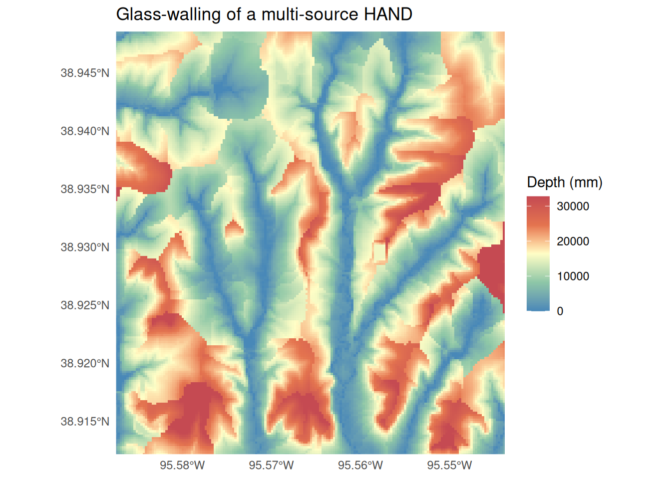
Glass Walling: A computational (and visual) mapping artifact in HAND-based models where simulated water reaches the outer boundary of a catchment mesh. Because the model boundary prevents lateral spread, further additions to height stacks upward, creating unrealistic vertical wall features at the edge of the domain.
GMS (Generalized Mainstems): An extension of the HAND framework that groups stream orders into distinct river branches. This optimizes FIM coverage along primary river corridors.
HAND (Height Above Nearest Drainage): A terrain model that calculates the relative elevation of every grid cell above its nearest drainage. It allows rapid estimation of inundation extents by comparing water stage directly to relative terrain heights.
HDF / HDF5 (Hierarchical Data Format): A file format used by HEC-RAS to store, organize, and read/write large spatial meshes, geometry, and dynamic time-series data.
HEC-RAS (Hydrologic Engineering Center’s River Analysis System): The standard software developed by the U.S. Army Corps of Engineers for performing 1D and 2D steady and unsteady hydraulic flow simulations.
HUC (Hydrologic Unit Code): a numerical identification system provided by the U.S. Geological Survey (USGS) that divides the landscape into nested drainage areas based on surface water features.
Hydrofabric (National Reference Hydrofabric): A standardized, nationwide spatial dataset defining stream networks, catchments, and channel geometry, providing a shared spatial backbone for hydrologic and hydraulic modeling.
InFRM (Interagency Flood Risk Management): A multi-agency collaborative group (FEMA, USACE, USGS, NWS) that establishes joint standards for flood risk modeling, data formatting, and web-map services.
Monolithic Processing (Version 2 / V_2): A version of the RAS2FIM method where an entire parent HEC-RAS model is simulated as one continuous system. This preserves the engineers model parameterizations before the outputs are clipped to match individual NWM catchments.
NWM (National Water Model): NOAA’s continental-scale hydrologic model that simulates real-time and forecasted streamflow for over 2.7 million river reaches across the United States.
Physical Subsetting (Version 1 / V_1): A version of the RAS2FIM approach that sliced large parent models into short, independent child models prior to simulation. While computationally faster, it created artificial boundary conditions that led to breakup errors.
RAS2FIM: An open-source Python tool built to automate the ingestion, execution, and translation of HEC-RAS models into standardized flood inundation depth grids aligned with National Water Model forecasts.
Rating Curve: An empirical or calculated relationship between water stage (elevation or height) and volumetric discharge (flow rate) at a specific cross-section or gauge location along a river.
RRASSLER: An R utility designed to spatialize legacy HEC-RAS models by extracting geometry and cross-sections into standardized geospatial formats linked to the national hydrofabric.
Strahler Stream Order: A numerical classification system that ranks river network complexity based on tributary branching, used in hydrography pipelines to partition stream networks into logical computational units.
Synthetic Rating Curve (SRC): A modeled stage-discharge relationship derived from geospatial terrain (e.g., HAND) or automated hydraulic runs rather than direct field measurements, allowing stage estimation on ungauged streams.

List of Figures

Chapter 1: Background

Abstract

The last decade has seen a near-exponential increase in the complexity and availability of Flood Inundation Modeling (FIM) methodologies. As the community transitions from reach-scale hydraulic modeling to national-scale geospatial forecasting, significant technical friction has emerged due to disparate data formats, model-specific driver requirements, and conflicting terminology used across the different efforts. This chapter traces the evolution of CONUS-scale FIM, from early Height Above Nearest Drainage (HAND) implementations to current multi-model ensembles. We identify a persistent “silo” effect where best-in-series models and the established standards take default precedence but remain operationally isolated.

Introduction

Flood inundation mapping, or the act of delineating the area under water, is a complex topic that highlights gaps in our understanding of the physical laws governing fluid dynamics, forces us to grapple with the technical friction of implementing that theory into operations, and antagonizes us with the need for decisive action in situations where every (in)decision has some degree of negative consequence to it. Of these challenges, the technical friction — the time and effort required to move from concept to a tangible map - has become increasingly pronounced over the past decade. This shift has been driven both by evolving geospatial modeling methods outlined in Figure 1 and by rapid advances in cloud-based computing paradigms. Geospatial flood modeling utilizes local, focal, and zonal operations commonly introduced in map algebra curricula. In contrast, hydraulic flood modeling typically solves forms of the shallow water equations for open channel flow, a methodology traditionally housed within engineering programs. Although broad-scale inundation mapping was once reserved for generalized analyses, pioneering demonstrations of the NWM-HAND-Synthetic Rating Curve framework by the NOAA Office of Water Prediction (OWP) sparked a dramatic surge in research. This momentum formalized and brought to publication numerous flood mapping methods (Afshari et al., 2018; Bhatt et al., 2017; Jafarzadegan & Merwade, 2019; Rebolho et al., 2018; Schumann et al., 2013). These methods may occasionally emerge from the same organization, but are more commonly tailored to specific use cases, utilize differing terminology, pursue distinct pathways toward technical realization, and, perhaps most frustratingly, require uniquely formatted drivers. It is this last point in particular, that each method currently requires its own dedicated input stream, that makes intercomparing models particularly challenging. To overcome that friction, we propose a framework for interoperable flood mapping efforts which unifies these discrete model into a set of common input choices which can be easily parsed and passed between methods.

Figure 1: Tracing the evolution of Flood Inundation Mapping (FIM) techniques from early 1D/2D hydraulic software (e.g., HEC-RAS) to modern automated and gauge-based FIM tools (e.g., OWP FIM, HAND frameworks). Node outlines distinguish open-source from closed-source iterations, while dashed lines mark key operational deployment milestones.

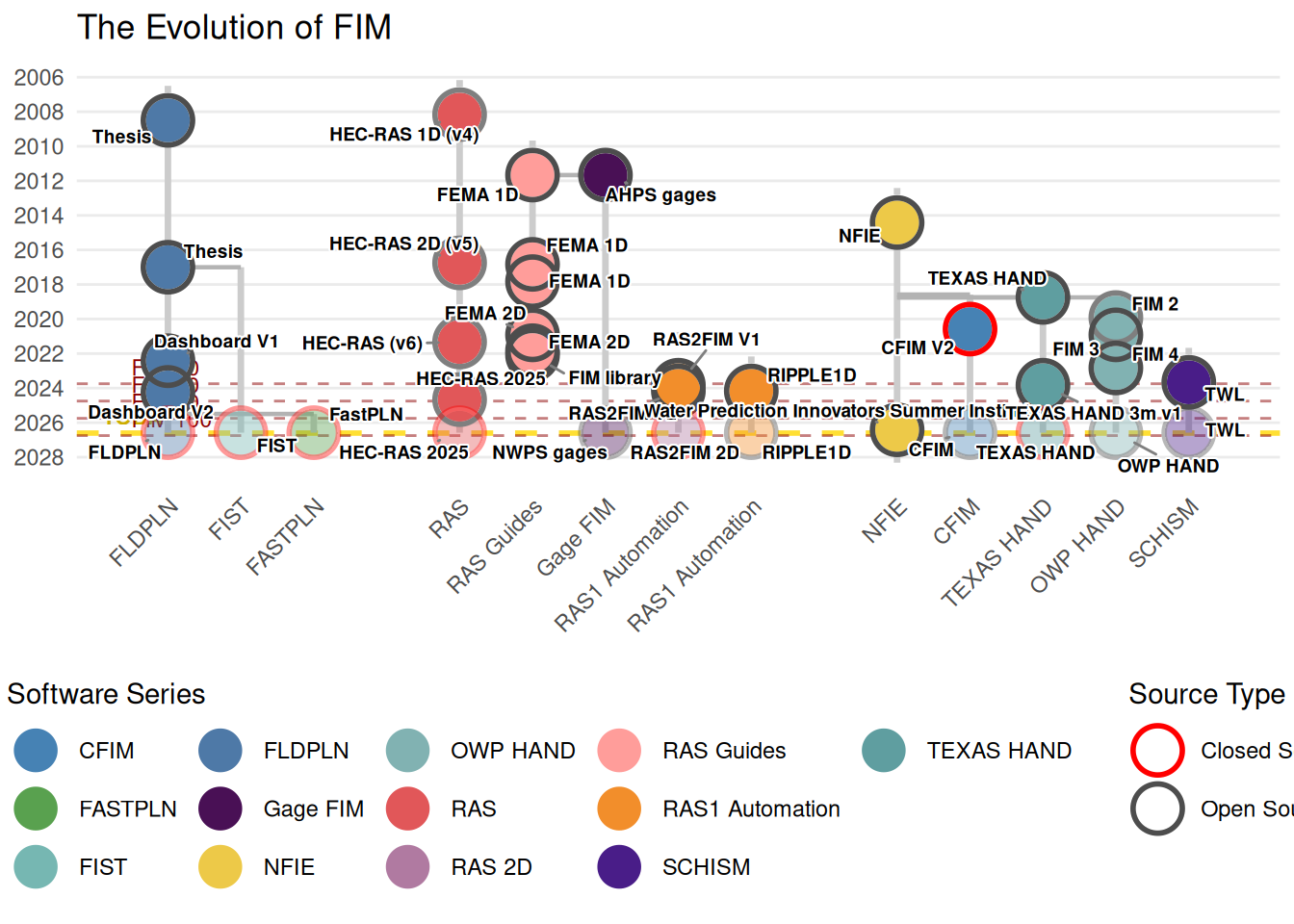
The Historical Trajectory of FIM: NFIE to FIM4

The National Flood Interoperability Experiment (NFIE) was a collaborative partnership across federal, state, and academic partners to explore how national-scale inundation mapping might be executed within the federal river forecasting enterprise (Maidment, 2017). In 2015, a “summer school” was convened in conjunction with the newly constructed National Water Center on the University of Alabama campus in Tuscaloosa, Alabama. Alongside federal staff and a cadre of professors and practitioners, a cohort of graduate students were able to demonstrate a potential pathway towards performant, street scale inundation predictions with a demonstration that with a Height Above Nearest Drainage (HAND) surface and associated basin, a synthetic rating curve could be constructed relating the hydraulic relationships with the geospatial model of terrain height (Nobre et al., 2011; Rennó et al., 2008).

After those initial successes, the Office of Water Prediction (OWP), academics, and private sector developers took ownership of flood inundation prediction and began operationalizing those research efforts into a more modern codebase. That transition saw the FIM program evolve from notebook and prototype code to a hardened and documented orchestration pipeline using ESRI ArcPy software to generate predictions, conversationally called FIM2. At the same time, academic efforts largely driven by Oak Ridge began exploring more performant ways to generate CONUS scale predictions using open source geospatial utilities within the context of the High Performance Computing environment Oak Ridge runs. This ultimatly resulted in the first, national scale HAND layers shown in Figure 2.

Figure 2: An image of the CONUS scale HAND map generated by the Oak Ridge CADES Condo cluster. In this map Dark blue represents low (0 meters) values for HAND and white represents high (~6000 meters). Green HUC6 overlays are shown indicating the domains users download these in. Image credit to cfim.ornl.gov.mhtml.

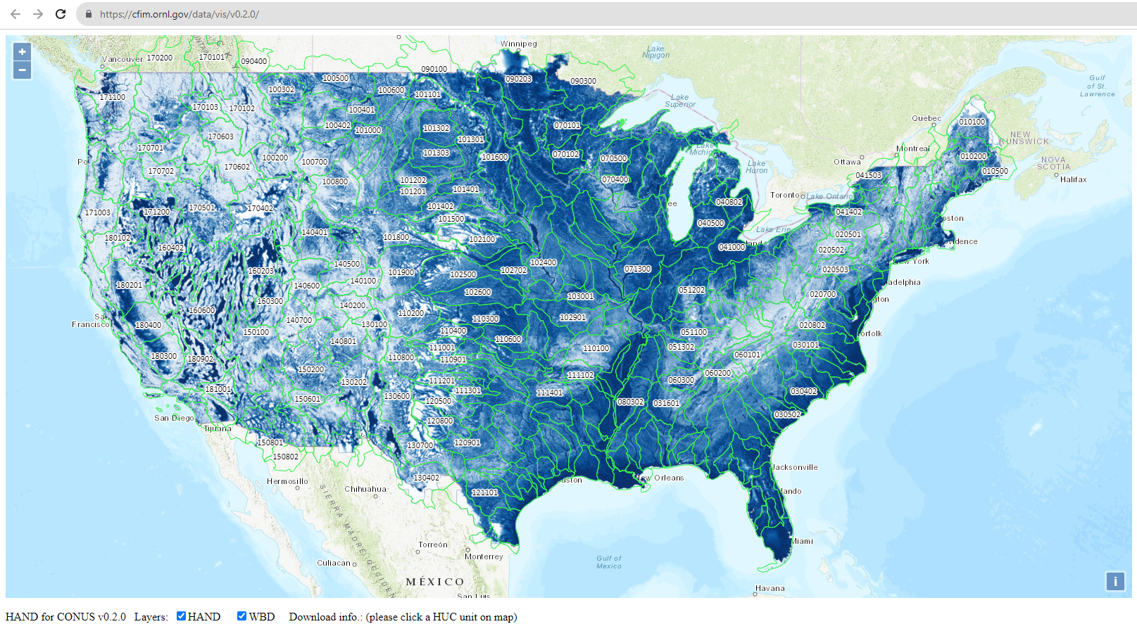
As the national scale FIM program developed and the use of the services gained more widespread adoption, the academic literature caught up to the state of the science and several of the most critical gaps in the approach became more prominent. Many correctly identified poor rating curve predictions as a large source of error (Ghanghas et al., 2022; Scriven et al., 2021), but evaluations typically failed to account for the complex forecasting chain and conflated the prediction of discharge with the skill of the FIM library. Visually, it also became apparent that the HAND domains were easily susceptible to “glass walling” as shown in Figure 3. This results because HAND domains are defined by watershed bounds, and so when the predicted height of the water meets those areas, the calculation and resulting maps can only expand upwards. When this glass walling occurs, it creates large visual anomalies and artifacts that immediately detract from the perceived trustworthiness of the map. To address this, new drainage paths were calculated so that a more consistent drainage source would be represented in a prediction, shown in Figure 4. This iteration also saw the code base transformed to open-source python implementation, conversationally refereed to as FIM3.

Figure 3: An example of ‘glass walling’ artifacts in a HAND surface. Artificial boundaries prevent the predicted inundation surface from flowing seamlessly across continuous terrain, creating unnatural boundary cutoffs.

Figure 4: An example of changes in library coverage introduced by the FIM3 mainstem technique, which incorporated additional libraries into the HAND processing methodology. The Full-Res library treats every flowline in the domain as a drainage source, whereas the mainstem representation isolates the largest levelpath as an independent volume within the broader library.

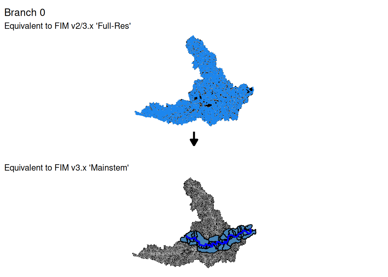
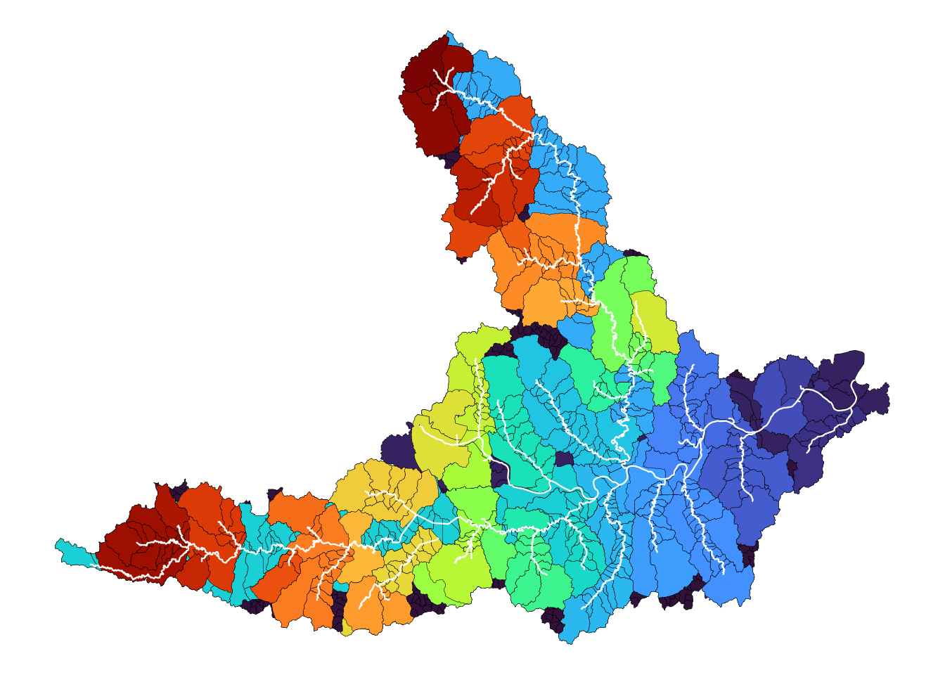
The next major iteration of the HAND code base saw more hardening and formalizing, including rebranding to the current day “NOAA-OWP/inundation-mapping” (FIM4) repository. It also saw a full expansion and generalization off that “mainstems” concept to each stream order in the network subset. Those (Strahler) stream orders were isolated into “branches”, and each branch could now comprise a holistic flood library. This “Generalized Mainstems” (GMS) approach provided improved skill at critical evaluation sites but saw the relative size of the national flood inundation library grow far larger than the visualization systems and operating costs could permit. These findings prompted the removal of that “Full Resolution” (now called “branch 0”) library in addition to all stream order 1-2 branches, drastically cutting down on library size while still maintaining explicit predictions for the major river network of the unit. Those mosaiced, overlapping branches are shown in Figure 5.

Figure 5: An example of the multiple branch FIM4 (GMS) library mosaic. The rainbow colors indicate specific levelpaths (hydrofabric relevent stream orders) that define FIM volumes relative to the hydrofabric defined levelpaths.

The Automation of Tradition: Advances in Automated Hydraulic Modeling

At the same time the advances in the geospatial flood modeling baselines were being developed, automation of hydraulic model FIM generation was also undertaken. The hydraulic modeling community maintain their own domain concerns, and the “gold standard” for accuracy codifies HEC-RAS as the de facto platform through which modeling activities take place. Traditionally, these models were manually intensive and reach-specific. However, the need for national coverage resulted in several options that automate the construction of FIM from these traditional engineering scale efforts.

The RAS2FIM system emerged to bridge that gap, automatically formatting and executing HEC-RAS 1D models using densified boundary conditions to generate standardized depth grids. Parallel efforts, such as the open-sourcing of ripple1d, exposed deeper model parameters, allowing for more defensible inundation libraries.

A Harmonious View of the Future

These rapid advancements in the tooling and techniques raise the ceiling in terms of capabilities, but by the same time also increase the needed technical skill and further push the implementations towards specialized formats and domain specific silos. We have reached a state where the various domains have favored models that are used as the gold standard benchmark against which other efforts are measured. These might provide the “best” (most true to our shared spatial reality) prediction of their system but without an interoperable layer or shared representation of the landscape, and an accessible means of executing, interpreting, and communicating those predictions we silo those advances and waste time, money, and talent that actively hinder forward progress on working our wicked problem.

The hydrofabric and the national water model provide a meaningful step forward towards harmonizing the prediction space, but only variations in pre-canned snapshots of mapping those predictions have been undertaken. It’s standard practice to use bulk mosaics and spatial priority lists to create a final inundation map, but this shared representation of landscape features presents an opportunity to more intelligently couple data, domains, and concerns

Conclusion: Painting the Future Landscape

The “Painting the Landscape” metaphor serves as a useful vision for future FIM operations. In this view, traditional career roles once drew hard lines between domain expertise and technical workflows. However, national-scale forecasting transcends these boundaries. It is no longer appropriate to isolate a “bad discharge forecast” from a “poor map”; the map consumer perceives only a single product. By harmonizing forecasts with HAND-shaped FIM libraries, it provides a bridge between research-grade modeling and the rapid cadence required for emergency response. As we move from an era of “model vs. model” to one of “model ensemble integration,” the focus shifts from the mechanics of map generation to the utility of the information in moments of crisis.

Chapter 2: RRASSLER

Abstract

HEC-RAS models are the benchmark for hydraulic modeling applications but, due to the way the data is passed to the application, format billions of dollars’ worth of data collection and analysis in forms not amenable to utilization outside the direct usage of a HEC application. Additionally, modeling efforts even up to today utilize legacy formats but in doing so lock those efforts behind technical walls as the evolution of computational sciences leads to new data and more efficient formats and processing architectures to store, distribute, consume, and archive the data that are critical to model execution. These advances often lead to new use cases for those data, which have a rich legacy and can be costly to collect, collate, and archive; but the form of that initial deployment sometimes makes integrating those original data into newer use-case workflows difficult. Those conflicting values create a need to make those model data more accessible and reusable, and a need to increase their findability and accessibility, a manifestation of the FAIR data principles. This chapter will demonstrate how legacy HEC-RAS one-dimensional model datasets are transformed and made more FAIR for uses in workflows across flood inundation mapping efforts.

Introduction

With the evolution of computation and scientific advances, it’s inevitable that the data and tools deployed at one point in time will eventually be depreciated in favor of more performant workflows, new data formats, and updated representations of the world. However, there’s still a huge amount of value, both direct and indirect, in reusing some of that data within the newer workflows. One example of this evolution can be found in the hydraulic modeling application and artifacts of HEC-RAS. Since its first release in 1995, users have created models using public and private data and countless hours of engineering scrutinization to generate the best possible purpose-built representation of the world. Like any model, some level of input manipulation is necessary to get the data into the specified mathematical format a model requires. Like most domain specific software, that manipulation results in data that modern geospatial data readers (such as GDAL) are unable to handle. This adds a great deal of overhead, both conceptually and technically, particularly when you take the standpoint of a model consumer.

F.A.I.R., or Findable, Accessible, Interoperable, and Reusable, are a series of adjectives describing principles and requirements for data users that, while broadly applicable to the entire life cycle of an analysis, are primarily aimed at enhancing how users programmatically interact with a data set (Wilkinson et al., 2016). Like any descriptor, there are varying intensities of FAIRness, and application specific requirements modify how FAIR a particular representation might be. Our intended data models are applications which use HEC-RAS data to automate FIM generation (RAS2FIM) and for more detailed cross section representations for use interoperability alongside a hydrofabric (Blodgett et al., 2021). This places extra emphasis on the Findability and Accessibility of those principles, while the extraction to point form facilitates reuse of that core data across other efforts.

HEC-RAS data is unique in that although it encodes spatial information, it is neither a standard spatial data format or strictly representative of space; meaning that the station distance and the cross section linestring distance are not necessarily equal to eachother. This makes using and accounting that data difficult. Additionally, archives of HEC-RAS models are rarely similarly formatted, with “value add” being specific to the archivist. There’s also no means of identifying whether a provided HEC-RAS model is already available, identical to an already aquired model, or is compliant for a given use case. Imagine a case where you have an algorithm you’d like to apply that needs some piece of data that a HEC-RAS model provides (e.g.: dishcarge, cross section form, rating curve). In theory, this could encompass all the different facets of a valid HEC-RAS model, but since models are typically designed for engineering and reach scales, where in space they represent is important. Archives such as the FEMA region 6 Base Level Engineering dataset serve models out in units that match HUC8 scales, although they also serve them out by political boundaries (counties) in some instances. For each unit, they provide three zipped archives. The most relevant for our task is the model data itself, sorted by reach name and model. The second separate zip archive includes model outputs in the form of rasters and geodatabases of spatial data (model cross sections and footprints). The last separate zip archive includes documentation on the model development itself. While all three of these archives are valuable, one would need to download all three datasets and perform manual interrogations and develop crosswalks if you’d like to use spatial queries or attribute filters to identify and access the relevant HEC-RAS model artifacts. Facilitating this sort of interaction is what we call “spatializing” a model.

Example uses of these models and the data include HEC-RAS itself, which needs all associated input files to rerun simulations and use that data as it was developed. Of course, one of the key pieces of data in a HEC-RAS model is channel geometry which could be reused across channel routing applications like T-ROUTE. Additionally, precipitation data and upstream discharge boundary conditions are stored in the rainfall files and would be invaluable in return period and design storm specifications. Our goal therefore is to more efficiently utilize that data across the different workflows that might be deployed. Several existing tools handle pieces of this workflow. For instance, USACE/mcat-ras, fema-ffrd/ras-stac, and psu-efd/pyHMT2D act as data readers, while utilitets like GitHub might accomplish versioning. However, none of these alternatives create a trackable artifact, convert legacy data into a modern spatial format, or seamlessly identify the model’s spatial extent. Therefore, the primary objective of this work is to prototype an approach that facilitates more FAIR patterns within and across the HEC-RAS data format. To do this, we develop and present an algorithm and workflow that ingests raw HEC-RAS models into a standard geospatial data format and anchors them to the National Reference Hydrofabric schema (Blodgett et al., 2021). This is provided in a documented R-based software package, RRASSLER. The remainder of this article will describe this algorithm in greater detail, demonstrate how the tool is deployed over a model, and outline how the resulting data structure and use cases are useful in bridging the scales of HEC-RAS and national scale FIM applications.

Methods (Software Design and Delivery)

Ingest logic

This section outlines the algorithm used to spatialize and account for a given model, elaborating on the package documentation. While it may be common to only have a single model that you’d like to interact with, it’s incredibly common to be given a zipped folder from a 3rd party that has many other vestigial data pieces and may be illogically organized or unsorted. Therefore, to start the program will recursively identify all files below the parent folder to identify the ones with a “.prj” extension. For each of those found files, we use the base name on that file to identify all files with a file extension that matches a “.g##” or “.g##.hdf”. The full list of files we identify is shown in Table 1.

Table 1: The grep expression, targeted model files, and their use in the HEC-RAS software that RRASSLER tracks as it creates a record.

File grep Pattern (# denotes single numeric wildcard)	HEC-RAS Model Use
.g##	Geometry definitions
.prj	Projection (can be non-standard proj4 string defined file)
.prj	Project (same extension, defines how RAS models are wired)
.p##	Plan file, used to drive the model
.f##	Steady flow file. Profile information, flow data and boundary conditions
.h##	Hydraulic design data file
.v##	Velocity file
.o##	Output file
.r##	Run file for steady flow
.u##	Unsteady flow file. Profile information, flow data and boundary conditions
.x##	Run file for unsteady flow
.dss	Data files
.rasmap	Output plan

If those files do not exist, the file we found is not part of a HEC-RAS model, and we move to the next file to process. If we do find a geometry (.g##/.g##.hdf) file, we parse out all .prj files with that base name to find the model units, which will always be found in a valid HEC-RAS project file, and projection files, which are rarely found (occurred for > 99% of the archive). If there is no projection file and no default projection provided, there is not enough information present to attempt to spatialize that model without an excessive amount of assumptions on our part. Because we do not want to use a model we are uncertain about, our workflow stops here and so the model files are placed in “unprocessed” for future investigation and manual intervention. If we found all the information we need, we attempt to convert those files into a table with columns for cross section number; station; x, y, and z of the point; and Manning’s n. If that conversation fails, that model is likewise placed in unprocessed. If it was successful and both the “.g##” and “.g##.hdf” files were found and converted, we select the table which has a lower normalized distance (the lowest deviation between station spesified distance and cross section linestring distance). Once we have the converted table, we attempt to create a footprint around the model bounds. If creating a footprint errors (occurred for ~0.2% of the archive), we append the model name with a “3”. If the footprint is generated, we attempt to join the model to a hydrofabric and select the first ID from the largest stream order. This workflow is diagrammed in Figure 6.

Figure 6: A data flow diagram following the project file through the core of the RRASSLER processing algorithm. Forks call out the different results of a parsing and the corresponding naming schema applied to the key.

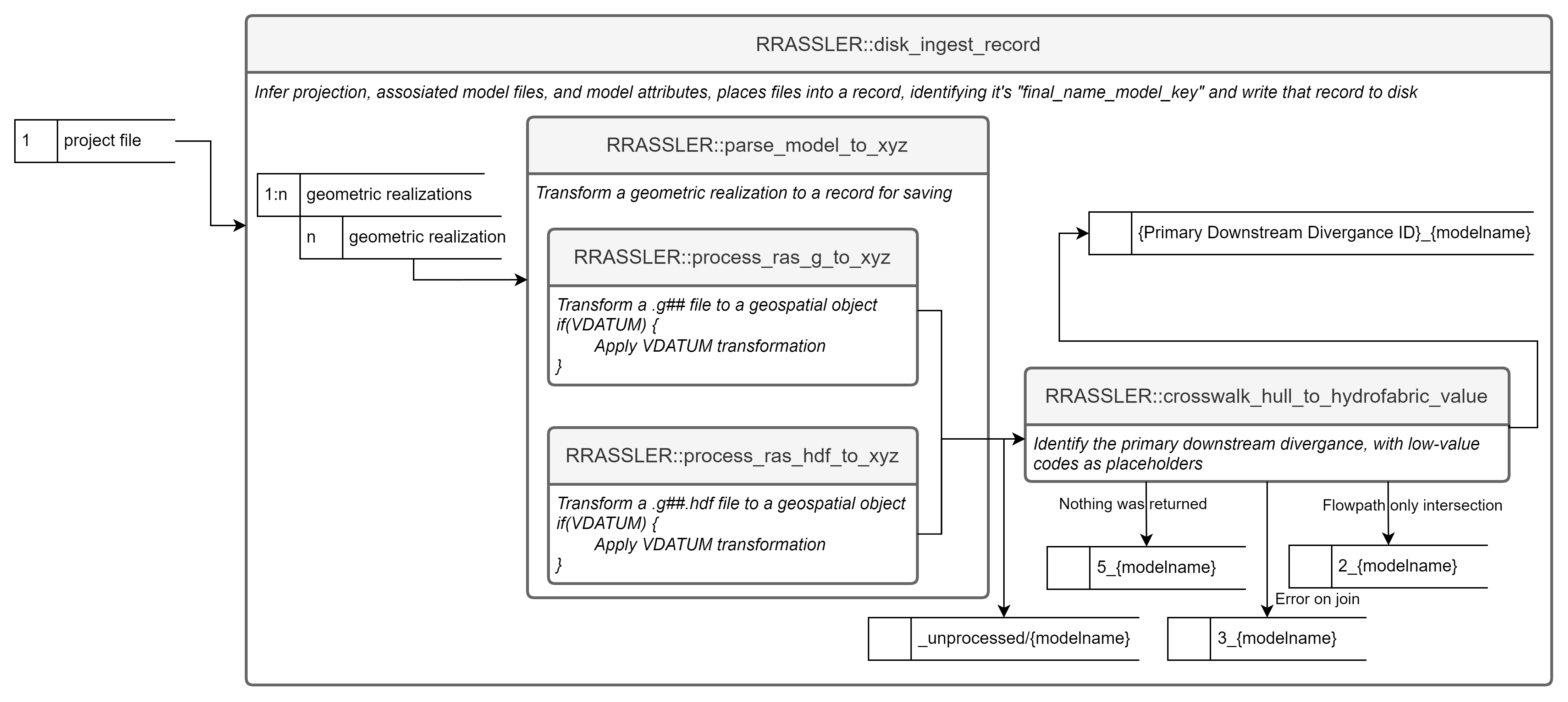
Note that this process and several of the other functions which take a path_to_ras_dbase argument are location agnostic. Therefore, although you will be operating over local files you may RRASSLE those into either a local directory or an S3 bucket using the same commands. RRASSLER also handles all “folder structure” differences between S3 protocols and disk representations, so the “bucket” argument can look just like a folder path or can be the “root” folder in an S3 URL and both are parsed out appropriately.

Results and Case Study

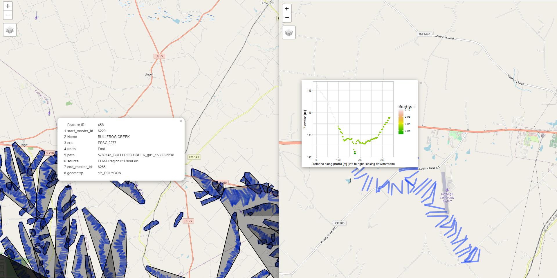
This section will describe the format of that RRASSLE’d directory and expand on several common use cases across CONUS scale applications. Additional resources on how these results are obtained and used are available in the package documentation. The RRASSLER catalog generates spatial data that includes the footprint of each record that contains pertinent, model level attributes as well as the name of the record that can be joined with the tracker sheet, shown in Figure 7. This gives us the accountability needed to deploy these HEC-RAS models in other workflows. Having constructed this, we’ll demonstrate two use cases where the RRASSLER database catalyzes those downstream workflows.

The first is a RAS2FIM run. RAS2FIM can iterate over multiple models but requires a homogeneous projection across the input data to generate the correct results and validating those inputs is beyond the scope of the tool. Without this RRASSLER catalog, users would have to parse the projection files in each database and remove the relevant files to their own directory for further processing. With a RRASSLER catalog, users can load the catalog and filter the records to the models within the domain of interest and grouped by projection and model unit. As one of the most common use cases for this data, RRASSLER also includes a wrapper, append_catalog_fields.R that can be used to construct the “OWP_ras_models_catalog.csv” that is used in that workflow.

Another common use case is the reuse of the channel geometry cross sections as transect for channel shape characterizations. The HEC-RAS and Hydrofabric data are complimentary but not immediately compatible and one of the most critical attributes needed for a hydrofabric transect is the stationing of that transect relative to the hydrofabric. However, HEC-RAS cross sections are relative to the models stationing and so they need to be cross walked to the new representation and renumerated so that each is uniquely indexed and addressable. RRASSLER facilitates this by allowing users to subset the cross sections to the desired streamlines and reindexed with the make_xs_hyfab_comp.R. function.

Figure 7: The RRASSLER outputs include transformations of the native HEC-RAS data to standard geospatial representations of those features. This enables users to interact with and identify the source HEC-RAS models using common geospatial software.

Discussion and Conclusions

Archives are only useful if the artifacts they collate are of value to end users. That value is diminished as end users experience technical friction integrating and interoperating between different databases into their applications. By spatially normalizing these models with accessible pointers back to source data, explicitly versioning different versions of the same model, and conflating that space into a CONUS scale framework, this work makes both individual archives and collections of archives more Findable, Interoperable, Accessible, and Reusable within native spatial applications like QGIS.

While RRASSLER successfully spatializes and exposes HEC-RAS model data, several operational limitations remain. Aligning model realizations across decades of software releases presents challenges; despite automated handling of standard edge cases and unit cohesion, spatial misalignment between digital elevation models (DEMs) and hydraulic models remains common. Minor surface variations frequently arise from differences in 3DEP timestamps, spatial resolutions, or reprojection order. Data collection and ingestion are a primary performance bottleneck. Because cloud-hosted archives lack standardized metadata, assessing a model currently requires downloading and local preprocessing. Transitioning to a cloud-native framework and enabling extraction of arbitrary cross-sections without full archive scraping would significantly improve data reusability. However, because executing a HEC-RAS simulation requires downloading the entire model, cloud-centric approaches offer the greatest utility during pre- and post-processing. Finally, RRASSLER was developed and validated exclusively on 1D hydraulic geometries; processing 2D models is currently unsupported and future efforts could be directed to address this limitation.

Software availability

Name of software: RRASSLER
Developer: National Oceanic and Atmospheric Administration (NOAA) Office of Water Prediction (OWP)
Repository: https://github.com/NOAA-OWP/RRASSLER
Programming language: R
License: Public Domain (US Government Work)
Software prerequisites: R Core Team (2024). R: A Language and Environment for Statistical Computing. R Foundation for Statistical Computing, Vienna, Austria. URL https://www.R-project.org/.

Chapter 3: RAS2FIM: A Python-based Framework for Automating Flood Inundation Mapping

Abstract

HEC-RAS Base Level Engineering (BLE) models serve as a foundational resource for flood risk assessment across the United States. However, these models are typically disseminated with a limited range of flows representing specific return periods. These discrete flow increments create significant gaps in rating curves, making the deployment of a Flood Inundation Map from that model difficult for operational and real-time contexts. This chapter presents RAS2FIM, a framework and tool used to generate flood inundation maps suitable for deployment using National Water Model (NWM) hourly operational streamflow forecasts. By automating the densification and extraction of flood depth rasters, RAS2FIM provides a programmatic means of tying legacy hydraulic engineering models to operational river forecasts.

Introduction

Hydraulic models, specifically the Hydrologic Engineering Center’s River Analysis System (HEC-RAS), provide an authoritative means of creating a Flood Inundation Map (FIM). One of the most common forms of these models are Base Level Engineering (BLE) models, which form the baseline for flood insurance studies and risk assessments. These models are typically provided using a range of discharges representing specific return periods. Because HEC-RAS is a hydraulic solver, the process of creating a map takes time and it’s common to separate the map and the model, and deliver both as separate archives so that users who are only interested in the map do not have to perform the computationally expensive step of running the model.

Another common method of creating a FIM comes from the National Water Model (NWM).The NWM is a continental scale model that provides reach scale forecasts of discharge at operational cadences. One of the primary uses of that model prediction is a Flood Inundation Map. This map is constructed by taking that discharge and calculating a stage that is used to create a water surface elevation prediction, and mapping that prediction to the landscape. This map is used to aid emergency response efforts and forecast impacts for alerts and to help save lives and property. To do so, that map needs to be provided quickly and relevant to the resolution of the prediction.

These two techniques for creating a flood map are not immediately compatible. Flood maps from BLE models are typically provided using a range of discharges representing specific return periods. While effective for regulatory planning, the discrete flows they model create large gaps in the resulting rating curves. This makes utilizing the model outputs difficult in that operational flood mapping context, which typically aim to resolve flood stages to half a meter. Furthermore, competent mapping and scaling of these models are often limited to manual interactions and small (watershed scale) domain sizes. This individualistic model access pattern, combined with the relative computational intensity that hydraulic solvers implement, results in an overly complex and intensive process that greatly increases the amount of investment needed to use these models as Flood Inundation Maps (FIM).

With no off-the-shelf solution for integrating these efforts, these challenges almost universally result in the disuse of these models and the underutilization of the billions of dollars of investment that went into the creation of them. We propose a framework to help bridge the gap between these distinct modeling paradigms, the hydraulic engineering scale and the continental hydrologic scale. To address this shortcoming, we present a framework and software solution, RAS2FIM, with the goal of demonstrating how these efforts can be reused and made interoperable within this operational mapping context. The software functions as an automated, open source HEC-RAS mapper that runs models to densify boundary conditions, creating FIM libraries tailored to NWM access patterns. The remainder of this chapter describes the framework RAS2FIM implements and examples of the outputs.

Methodology and System Architecture

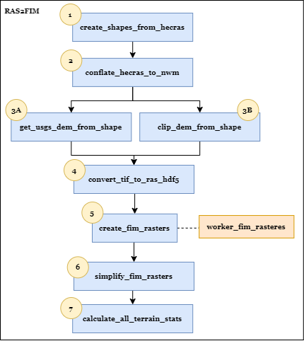
The RAS2FIM framework utilizes HEC-RAS in a one-dimensional steady-state hydraulic analysis to construct a flood inundation library. The workflow is orchestrated via a series of Python scripts that execute seven sequential steps to transform raw HEC-RAS models into flood inundation libraries usable by the National Water Model. That sequence is diagramed in Figure 8, and includes the major steps and conceptual choices a user can make.

Figure 8: A functional flow diagram of the major steps of the RAS2FIM pipeline. Steps are executed sequentially for all models and each function is labeled with the primary objective of the step.

Geometric Extraction and Hydrofabric Conflation

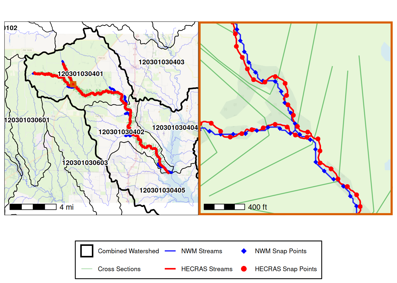
The RAS2FIM pipeline starts by scraping the input directory to identify relevant HEC-RAS projects. The system determines the geometry set in the active plan as defined by the HEC-RAS model and, if necessary, computes the plan to generate the required Hierarchical Data Format (HDF) files needed by more modern versions of the HEC-RAS utility. From that transformation, stream centerlines and cross-section vector geometry are extracted and merged into shapefiles to establish the spatial footprint of the hydraulic models. To identify the portions of the HEC-RAS model that are relevant to the NWM forecast, the NWM streamlines that intersect the HEC-RAS model footprint are selected and points are placed along it at 150-foot intervals along both lines. Points from the NWM streamlines are snapped to the HEC-RAS river points and the model which has the greatest count of snapped points becomes the conflated feature to use, as shown in Figure 9. This process also identifies what cross sections of the parent HEC-RAS model are most up- and downstream of the conflated reach so that excessively long models can be appropriately trimmed. This subset of the parent HEC-RAS model now forms the definition for the child HEC-RAS model we will use to create our inundation models.

Figure 9: A graphical representation of the stream conflation process demonstrating how overlapping models at confluences are conflated to the National Water Model streams.

Terrain Acquisition and Processing

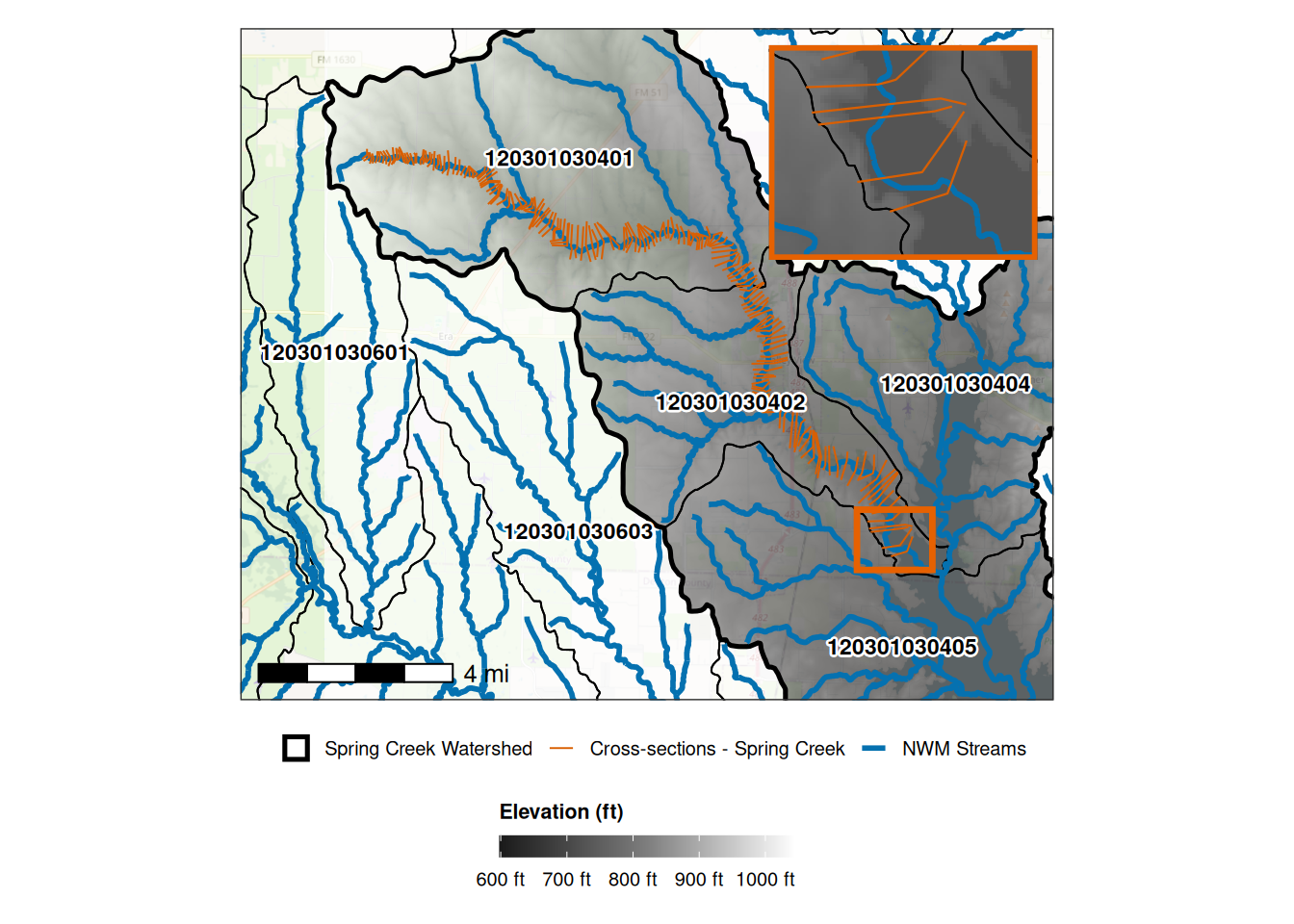
If a user does not supply a terrain file, RAS2FIM automatically acquires bare-earth DEMs via the United States Geological Survey (USGS) 3DEP service as shown in Figure 10. The data is retrieved for relevant HUC-12 watersheds, reprojected to the coordinate reference system of the HEC-RAS model, and converted to the requisite HDF5 compliant form for HEC-RAS terrain files.

Figure 10: An example of the automated DEM collection process that is used if users do not supply a DEM to map over. Note that the utility will provide comprehensive coverage across the entire domain. Note that because the model hull overlaps small areas of external HUCs (inset), those basins are included in the processing.

Synthetic Rating Curve Generation

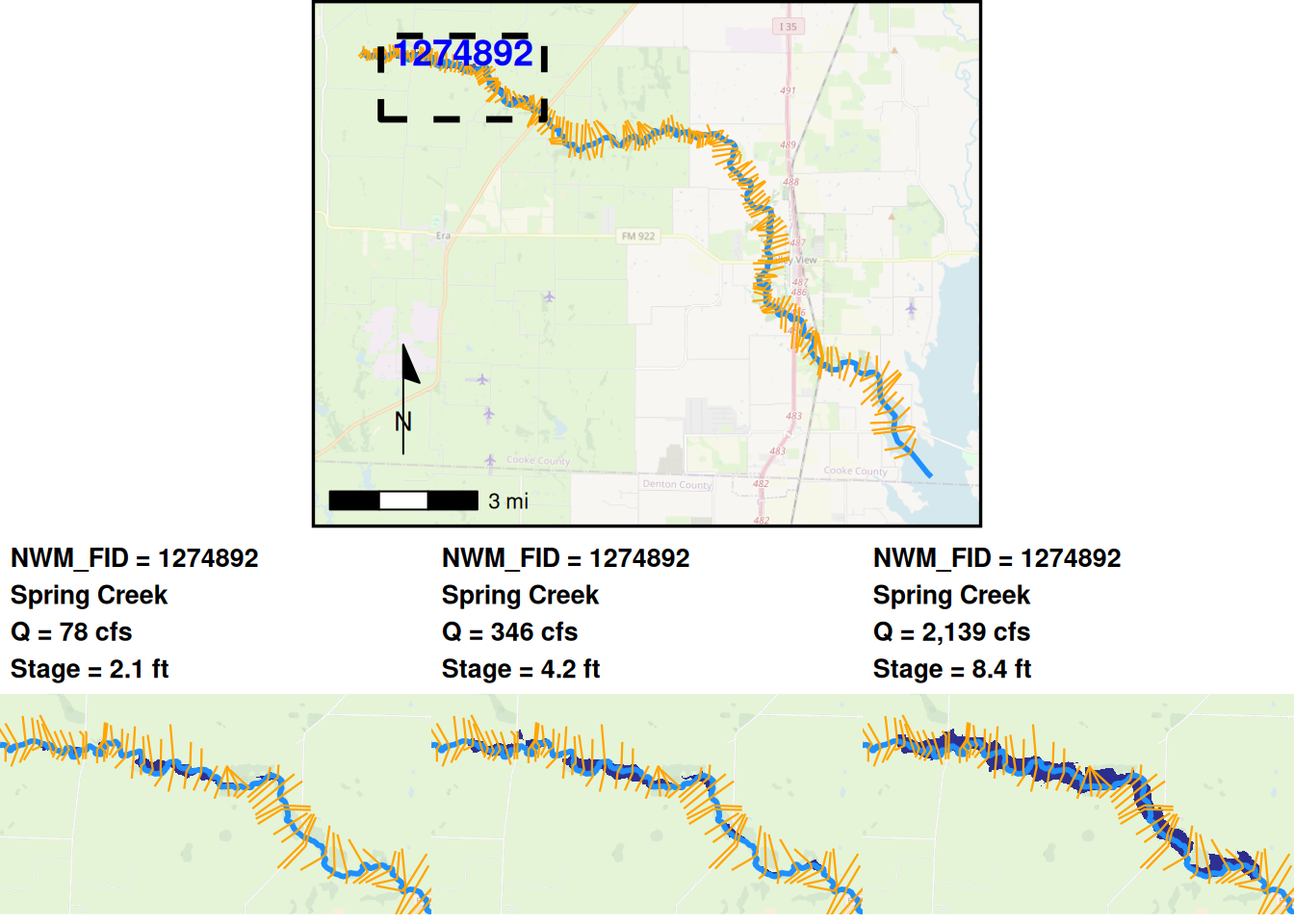
To generate a “synthetic rating curve” critical to the definition of a flood inundation library, the model is executed across a range of discharges. The “parent” HEC-RAS model is treated as a monolith, where input model boundary conditions are densified to create tighter increments of flow. The system takes the maximum flow from the conflated model, multiplies it by a factor of 1.2 (a factor of safety), and divides the result into 75 evenly intervaled flow values to run the model, visualized in Figure 11. For the analysis, all flow is considered sub-critical, and downstream boundary conditions are set assuming a normal depth with an energy slope of 0.5%. From each run, a reach-averaged depth is calculated for each discharge. This data results in a first-pass rating curve.

Figure 11: An example of the feature conflation performed to slice up the parent model into the constituent child model. For the particular NWM feature (5791020), three different depictions of the resulting flood map and reach averaged rating curve calculation are shown across the bottom, against the context of the larger models that were run in the RAS2FIM system.

Inundation Mapping and Simplification

Using those first pass rating curves, the flow needed to create the more evenly intervaled FIM access patterns is calculated and a second HEC-RAS simulation is executed using the interpolated flow rates. The RAS Mapper engine is utilized to generate inundation boundaries for those equal-interval stages. To ensure the resulting data is suitable for web-based dissemination, the output rasters undergo a simplification process compliant with Interagency Flood Risk Management (InFRM) standards. The depth grids are re-projected to WGS84 Web Mercator (EPSG:3857), resampled to a 3-meter cell size, and converted to 16-bit unsigned integers. In this format, the integer values represent decimeters of depth (metric) or tenths of a foot (SI), significantly reducing file size while maintaining vertical precision (Wallace, 2022).

Map Quality Assessment

The framework includes a module to calculate terrain statistics, addressing potential discrepancies between the terrain used in the mapping process (either user supplied or USGS 3DEP terrain; Figure 8 step 3A or B) and the terrain used to develop the HEC-RAS geometry as extracted from the cross section. The script compares those elevations to calculate the vertical error. If the median, mean, or standard deviation of the error exceeds a user defined acceptance threshold, the resulting FIM library could be flagged for potential exclusion.

Results

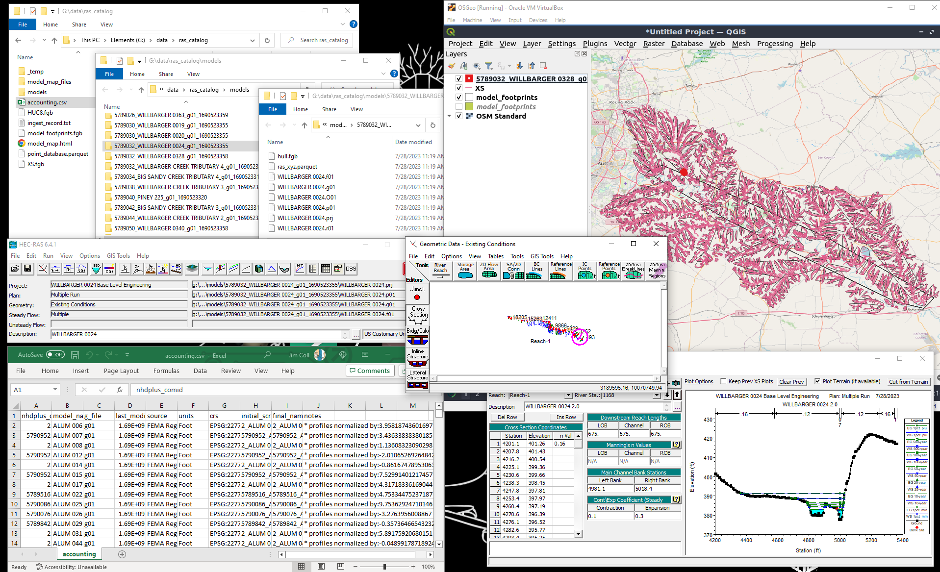
The results of a sample RAS2FIM run are included in the repository and demonstrate how the single model used in this test example is conflated and generates the described data. A mosaic of inputs and outputs for a full HUC8 process output is shown in Figure 12, where HUC 12090301 was processed from end-to-end.

Figure 12: A screenshot mosaic of the various forms and outputs of a RAS2FIM execution, highlighting the child HEC-RAS models created in step 4 (Figure 8), the reach averaged rating curve from step 6, and the footprints from the models shown as red polygons, the maximum potental flooding extent of the underlying model.

Discussion

The RAS2FIM implementation conflates model and map space by making several critical assumptions regarding model structure. The program is currently only constructed to execute over steady-state, one-dimensional HEC-RAS models; unsteady flows and two-dimensional models are not currently supported. While the hydraulic calculations respect bridges, culverts, and inline structures, the processing omits storage areas and lateral structures—components that can significantly alter flow dynamics and inundation results when present. Furthermore, programmatic bulk processing requires all input data to share a uniform geographic projection to avoid spatial errors during execution.

Methodologically, conflating the HEC-RAS crosswalk with National Water Model features introduces spatial and hydrologic limitations. The utility attempts to pair each model with an appropriate NWM feature even when point-snap density is low, which risks misalignments around complex geometries such as contributing branches or river confluences. In instances where two models tie for a single forecast feature, the algorithm arbitrarily defaults to the first model processed. Finally, when parent HEC-RAS models are exceptionally long relative to the corresponding NWM reach, or when substantial lateral inflows are present, the discharge may be under-parameterized. This unaccounted-for volume can cause the resulting maps to underpredict inundation extent.

Conclusion

RAS2FIM demonstrates a free and open, programmatic means of reusing compliant HEC-RAS 1D models as flood inundation maps suitable for deployment within the NWM operational flood inundation workflows. By automating the translation and execution of engineering scale hydraulic models to a CONUS scale prediction framework, compatible Flood inundation libraries can capitalize on the high-fidelity flood knowledge of these efforts without the tedious and error prone processes of the HEC-RAS point-and-click interface. However, the utility of these output libraries is constrained by spatial alignment challenges and structural simplification, as the current framework is restricted to steady-state, 1D models and omits complex features like lateral storage areas. Consequently, operational applications must account for potential underprediction of inundation extents near complex channel geometries and reaching boundaries with unparameterized lateral inflows.

Software Availability:

Name of software: RAS2FIM
Developer: National Oceanic and Atmospheric Administration (NOAA) Office of Water Prediction (OWP)
Repository: https://github.com/NOAA-OWP/ras2fim
Programming language: Python
License: Public Domain (US Government Work)

Software prerequisites:

• HEC-RAS: The software relies on the HEC-RAS computational engine (Version 5.0.7 or later) developed by the U.S. Army Corps of Engineers (USACE).
• OS: Windows 10/Server (required for HEC-RAS COM automation).

Data Availability:

The datasets generated and/or analyzed during the current study are available from the following sources:

• HEC-RAS Models: The local hydraulic models used as input were sourced from FEMA Region 6 and the Iowa Flood Center.
• Hydrography: The National Water Model (NWM) stream network data is available through the NOAA Office of Water Prediction.
• Terrain Data: Bare-earth digital elevation models (DEMs) were accessed via the USGS 3DEP Web Coverage Service (https://elevation.nationalmap.gov/arcgis/services/3DEPElevation/ImageServer/WCSServer).

Chapter 4: Evaluating the Senativity of Model Breakup Strategies Using RAS2FIM

Abstract

The integration of legacy HEC-RAS hydraulic models for use in National Water Model (NWM) Flood Inundation Mapping (FIM) workflows provides a scalable pathway to capitalize on these hydraulic-scale models at the Continental United States (CONUS) scale. However, the methodology used to “break” large, complex hydraulic models into segments aligned with NWM reach IDs introduces potential errors. This chapter evaluates two distinct strategies developed within the RAS2FIM framework: Version 1 (Physical Subsetting), which creates standalone “child” models, and Version 2 (Monolithic Processing), which extracts data from full model simulations. We analyze the error introduced in this process by executing these two approaches over the same parent model and evaluate the differences in stage from the resulting reach-averaged synthetic rating curves (SRCs). Results show that the physical subsetting offers improvements in computational efficiency and increases in potential inundation map coverage but introduces artifacts at high discharges, particularly within the lowest stations of the model due to truncated boundary conditions and loss of downstream controls.

Introduction

Historically, Flood Inundation Mapping (FIM) has been a localized, gauge-dependent endeavor. The advent of the National Oceanic and Atmospheric Administration (NOAA) National Water Model (NWM) has shifted this paradigm by providing hourly streamflow forecasts for over 2.7 million reaches across the United States, greatly increasing the predictive potential and enable stream level access to critical inputs needed to execute and access flood inundation libraries. To translate these flows into actionable depth maps, the RAS2FIM framework was developed to automate the conversion of existing HEC-RAS models into NWM-compatible flood libraries. A primary challenge in this automation is the spatial mismatch between the hydrofabric used by the NWM and the river stationing of legacy HEC-RAS models. This requires a strategy to associate specific model reaches with specific NWM reach IDs.

However, conflating these hydraulic models, which are typically constructed for local consumption, is not a direct process. HEC-RAS models are typically a higher resolution than the CONUS-scale framework used in the national water model, and conflating them to this coarser resolution is not a standardized or straightforward process. This chapter investigates the hydraulic implications of two conflation strategies, quantifying the error introduced when a continuous hydraulic model is segmented prior to its use.

Methods

The RAS2FIM Framework

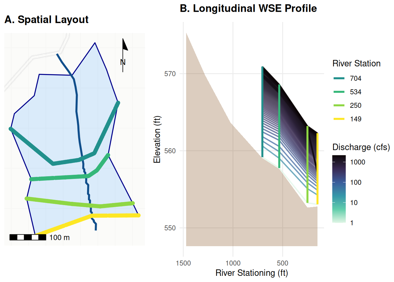
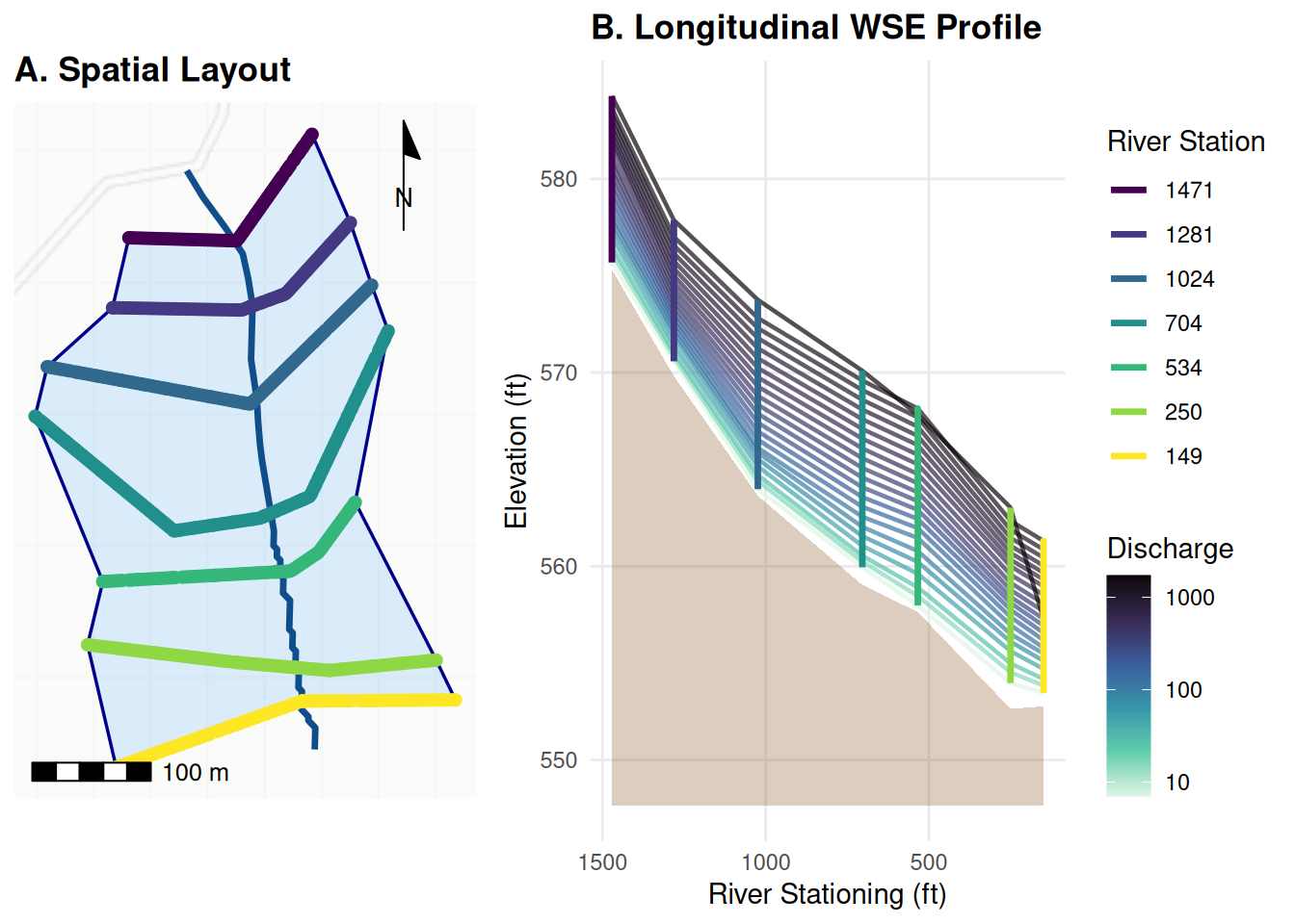
RAS2FIM utilizes Python-based automation and the HEC-RAS API to process potentially thousands of models. Version 1 (V_1) of the workflow involves conflating parent HEC-RAS models to the NWM forecast features, generating subset children models relative to that feature, and running the model across a range of discharges before averaging out the resulting model to a reach average rating curve and generating the resulting inundation maps shown in Figure 13. Version 2 (V_2) (Figure 14) treats each model independently and attempts to apply reach averaging during execution.

Version 1: Physical Subsetting (Child Models)

In V1, the system identifies the “parent” HEC-RAS model most representative of an NWM reach. It then performs a physical “slice” of the geometry, extracting the relevant reach plus a buffer of two cross-sections upstream and downstream. These slices are saved as independent HEC-RAS projects. In that process, a normal energy grade line is used to set the downstream boundary condition.

Figure 13: A top-down (A) and longitudinal plot (B) of the model domain and the water surface elevations predicted in a V_1 RAS2FIM configuration.

Version 2: Monolithic Processing

Version 2 maintains the integrity of the original “parent” model. The entire model is simulated as a single monolith. Post-simulation, the depth rasters and rating curves are clipped and indexed to the NWM hydrofabric. This approach preserves the longitudinal hydraulic connectivity and any backwater effects present in the original engineering study.

Figure 14: A top-down (A) and longitudinal plot (B) of the model domain and the water surface elevations predicted in a V_2 RAS2FIM configuration.

Metrics

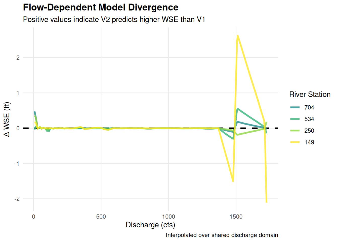
To quantify the deviations this process introduced, we compared V_1 and V_2 outputs using the National Water Model feature-based access patterns, comparing the residual water surface elevations (\Delta\text{WSE}) between versions (\Delta\text{WSE} = \text{WSE}_2 - \text{WSE}_1) to identify where and how these approaches vary, both spatially and hydraulically.

Results

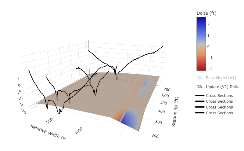
Plotting the surface differences between V_1 and V_2 as shown in Figure 15 indicate a consistent positive bias, where the monolithic V_2 approach generally predicts higher water surface elevations than the subsetted V_1 approach but is flow-dependent. To emphasize this behavior, it is useful to plot the normalized (to a single spatial dimension) form of the model with the rating curve as a 3D surface, shown in Figure 16. This visual helps contextualize both the computational surface HEC-RAS represents and the variations that were found between the different versions. It shows that while the models remain relatively aligned at lower discharges where flow is contained within the primary channel, the error magnitude increases as discharge approaches the upper limits of the model. Spatially, these deviations are concentrated at the downstream-most stations of the models.

Figure 15: Variations in water surface elevation by cross section across the shared range of discharges.

Figure 16: A 3D plot of the changes in stage introduced between the two approaches. Downstream and high discharge areas exhibit the largest variations

Discussion

This comparison reveals distinct hydraulic deviations driven by the choices in model conflation and processing. While all models are unique, the variations found in this model indicate meaningful variations in the different ways hydraulic models are constructed and executed. Plotting the surface differences between the two versions indicates a positive bias across this model where the monolithic V_2 approach predicted higher water surface elevations than the subsetted V_1 approach and was discharge dependent. This bias was not spatially uniform but increased as the model length increased and were concentrated at the downstream-most stations. The V_1 workflow, by virtue of its smaller, independent “child” models, required less processing time per simulation (01 mins 42 secs vs 04 mins 30 secs). However, the loss of longitudinal connectivity and the resulting 1–2 foot elevation errors suggest that these efficiencies come at the cost of significant accuracy given the half-foot intervals that the resulting Flood Inundation Library aims to represent. This is perhaps unsurprising given the control downstream boundaries have on subcritical flow calculations.

Conclusion

The transition from physical subsetting (V_1) to monolithic processing (V_2) represents a significant methodological deviation that has meaningful implications in the accuracy of the resulting flood map. While V_1 is computationally cheaper for localized updates, the “breakup error” introduced by physical segmentation can exceed 1-2 feet in elevation at peak discharges. For national-scale implementation, we recommend the V_2 monolithic approach as the standard for generating Synthetic Rating Curves. V_1 should be reserved for high-gradient, headwater reaches where downstream boundary conditions have minimal impact on upstream profiles, or when more complete coverage of the domain is a primary objective.

Chapter 5: Assessment of the Impact of Access Patterns on Categorical Flood Mapping

Abstract

The libraries of predictions generated by a Flood Inundation Model (FIM) are only as useful as the access patterns they expose. Traditional accuracy assessments tend to favor large geographic processing aggregations, rely on a handful of well-cited metrics to assign model skill, and typically utilize the most familar pathways to access a layer. This paradigm inherently favors libraries and evaluation frameworks that cater to the entirety of the modeling pipeline or models operating under well-aligned drivers and favorable locations. Consequently, those standard evaluations gloss over skillful mapping workflows and incorrectly penalize libraries that would otherwise perform well by decoupling hydrologic, hydraulic, and geospatial drivers from the map creation process. By exercising greater intentionality in how we access these libraries, we can maximize the utility of distinct FIM approaches. This shifts the focus from the isolated mechanics of modeling and forecasting to the effective retrieval and communication of generated maps.

Introduction

With the operational deployment of the National Water Model (NWM), Flood Inundation Mapping (FIM) has evolved to provide predictive coverage for 100% of the CONtiguous United States (CONUS). For a map to be useful it should reflect spatial reality and one of the ways that reflection of reality is reported is an accuracy assessment, comparing the generated map to a known ground truth or measurement. However, most assessments gloss over or conflate the model prediction pipeline and aggregate many different flood maps into a singular score (Aristizabal et al., 2023; Baruah et al., 2025).

This standard practice in assigning a single value loses the ability to distinguish skill across space and flow regimes. More critically, these assessments evaluate the entire modeling pipeline, from the prediction of discharge to the routing of mass to the energy balance of a water surface profile (hydrology, hydraulics, and mapping) as a single intertwined unit. If a model’s underlying rating curve or routing is off, the resulting map is unfairly penalized, even if the spatial representation of that specific volume of water is otherwise highly accurate. This risks discarding useful maps or placing unwarranted trust (or lack therein) in the methods that placed that map maps that perform well under specific instances but fail to capture the integrated system.

To address this shortcoming, we should explicitly consider the “access pattern” used to create a map. We define an access pattern as the specific methodological logic used to query, retrieve, and translate a hydrologic condition (such as a predicted gauge stage) into a corresponding spatial map. By accounting for the access pattern, we can decouple hydrologic and stage translation errors from the spatial mapping skill of the library itself. A more nuanced, optimized access pattern can significantly increase the apparent accuracy of a map by circumventing the cascading uncertainties associated with structural model biases, datum differences, and integrated hydrologic/hydraulic modeling.

To perform this assessment, we use three different forms of a stage based flood inundation library. Stage based libraries, particularly those that include layers representing the ‘minor’, ‘moderate’, and ‘major’ flooding catagories called out in gauge impact statements, are an accessable entry point for the broader public to assess the impending danger a flood might represent. The first, and most conventionally trusted source of reference truth are the gauge based library from the Partner FIM repository provided by NOAA. These libraries are commissioned by regional, state, and local partners and are typically generated specifically for sites which host a river monitoring gauge. These receive special attention and QA/QC as they are more limited in scope than automated alternatives such as base level engineering models. Because these are extensively validated and frequently consulted during events, practitioners place a lot of weight in the predictions they make. The objective of this analysis is to quantify the performance of several categorical FIM libraries against the AHPS reference and demonstrate how an informed use of library access helps improve the skill of the prediction.

Our second form of categorical flood maps are generated from FLDPLN (“Floodplain”) libraries. FLDPLN is a model that provides continuous stage-based local flood extent and depth grid estimates (Kastens, 2008). To transform these estimates into a categorical prediction, the stage of the gauge uses FLDPLN’s intrinsic stage/volume relationship to interpolate stage (holding volume constant) up and downstream from the target gauge as needed to generate localized stage values sufficient to cover the study site. These resulting inundation maps are merged, cropped and indexed to the network much like the Partner FIM.

Our third source of categorical flood map is derived from the Office of Water Prediction (OWP) HAND (Height Above Nearest Drainage) libraries. These libraries provide predictions of both a discharge and a stage and are scoped for the National Water Model forecast elements. The objective of this analysis is to quantify the performance of HAND and FLDPLN against the AHPS ground truth using the MNTK1 gauge site domain as a case study.

Methods

Flood forecasting is a complex workflow even at the site-specific level. Geodesic measurements, unit conversions, projection handling, and feature indexing all require intentional handling to ensure a correctly realized system. These cascading variables end up confounding the mapping process and introduce their own errors when we attempt to quantify the skill of a prediction. The end-user of a flood map primarily cares about how true the prediction is to their spatial reality, and will quickly dismiss an entire output if that expectation is not met, regardless of the underlying model’s merits. To isolate the spatial skill of the map libraries from these cascading modeling concerns, the categorical flood maps were compared using two distinct access patterns:

Direct Numerical Stage Access - Baseline Deployment Pattern

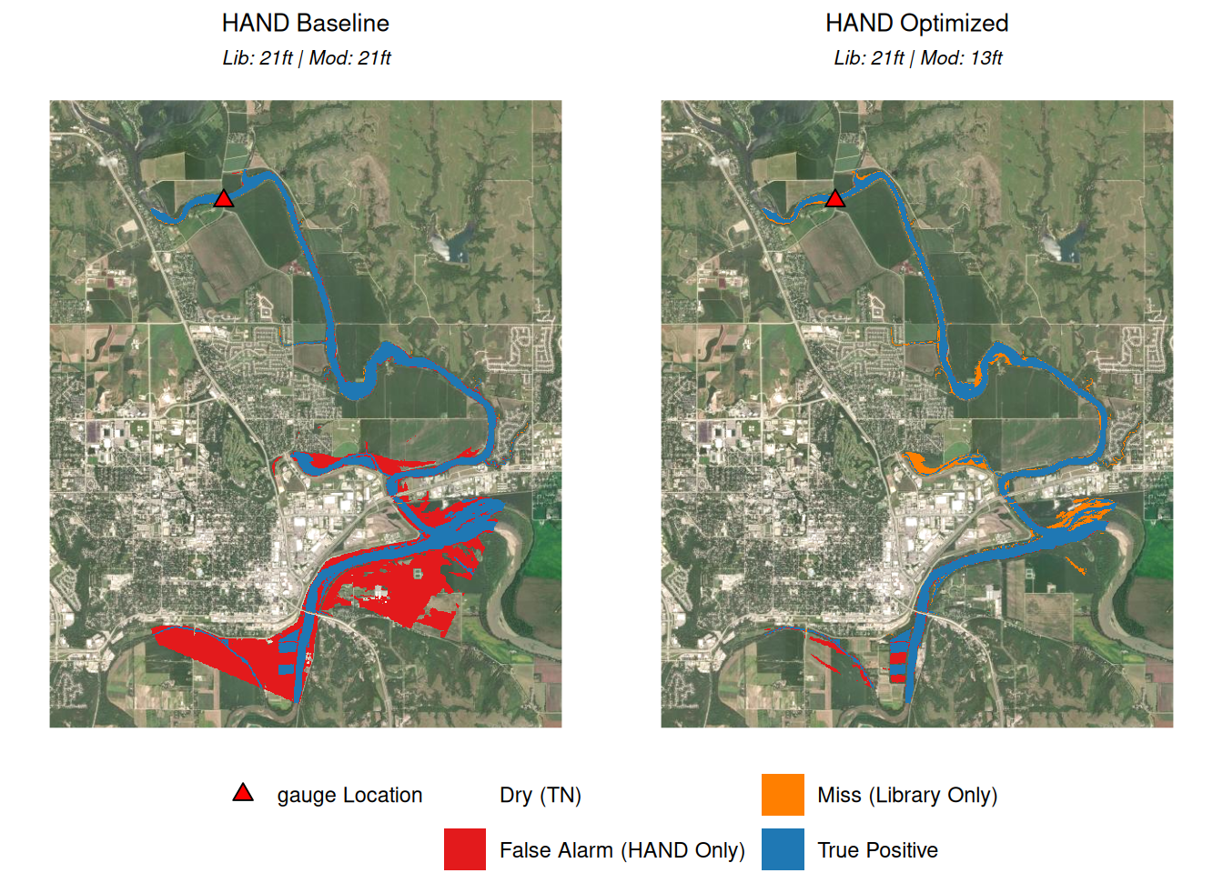
The most traditionally deployed method is a 1:1 numerical mapping between the reference library and the evaluated library. Under this access pattern, the exact numerical value of the gauge stage is used to access the corresponding flood map for comparison. For example, the spatial extent of the 18-foot AHPS reference map is compared directly against the spatial extent of the 18-foot HAND map and the 18-foot FLDPLN map. This serves as the baseline assessment, demonstrating how the models perform when structural biases (such as rating curve deviations or differing datum assumptions) are left uncorrected.

Mapped Stage Access - Optimized for Mapping

To circumvent library-specific variations and structural biases, we applied an optimized “mapped stage” access pattern. Instead of forcing a direct numerical match, this approach acknowledges that an 18-foot stage in one model’s hydraulic reality may correspond to a different numerical stage in another model due to differing underlying terrain assumptions or volume allocations. To execute this, the reference stage was systematically compared against a range of candidate stages in the evaluated library (FLDPLN and HAND) to identify an optimal offset. The evaluated map that generated the highest F1 score against the AHPS reference map was selected as the reference “mapped stage.” By shifting our access pattern to select the most spatially appropriate library map for the shared domain, we can evaluate the capability of the library independent of its numerical stage assignment.

Metrics

While the act of calculating accuracy is a mathematical exercise, a great deal of user-specific judgment, preference, and objective is used in selecting a metric to report. Because flood inundation is an inherently imbalanced classification problem—where the “flooded” pixels make up a very small minority of the total mapping domain—metrics that heavily weight True Negatives (TN) inflate apparent model performance. To accurately reflect model skill, we rely on two widely accepted metrics (eg: Nikrou et al. (2026) that focus strictly on the positive (flooded) class: the Critical Success Index (CSI) and the F1 Score. F1 is the harmonic mean of precision and recall while CSI is the more simplistic intersection-over-union (IOU). CSI penalizes more heavily for misses (FP & FN). The formulas, score range, optimal (ideal) value score, and formula are presented in Table 2.

Table 2: Evaluation metrics used to assess categorical flood map performance, where TP = True Positive, FP = False Positive, and FN = False Negative.

Metric	Range	Ideal	Formula
CSI	0 to 1	1	\frac{TP}{TP + FP + FN}
F1	0 to 1	1	\frac{2TP}{2TP + FP + FN}

Case Study: Big Blue River near Manhattan, Kansas (MNTK1)

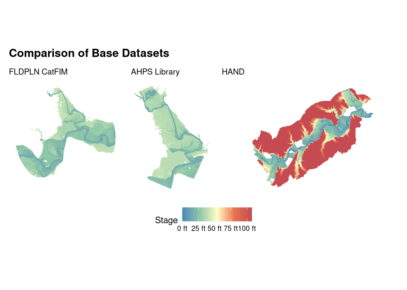
To demonstrate the impact of access patterns, this study utilizes the domain surrounding the MNTK1 stream gauge as a case study. MNTK1 is operated by the U.S. Geological Survey (USGS ID: 06887000) and represents the Big Blue River just north of Manhattan, Kansas. The site is situated less than two miles downstream of the Tuttle Creek Dam. This area features several designated impact stages and serves as a useful study area, as several categorical FIM libraries overlap here. The categorical FIM libraries evaluated in this study are visually compared in Figure 17.

Figure 17: A visual comparison of the different categorical flood libraries used in this demonstration, FLDPLN CATFIM (left), AHPS partner FIM (middle), and OWP HAND FIM4 (right).

Results

Direct numerical stage access

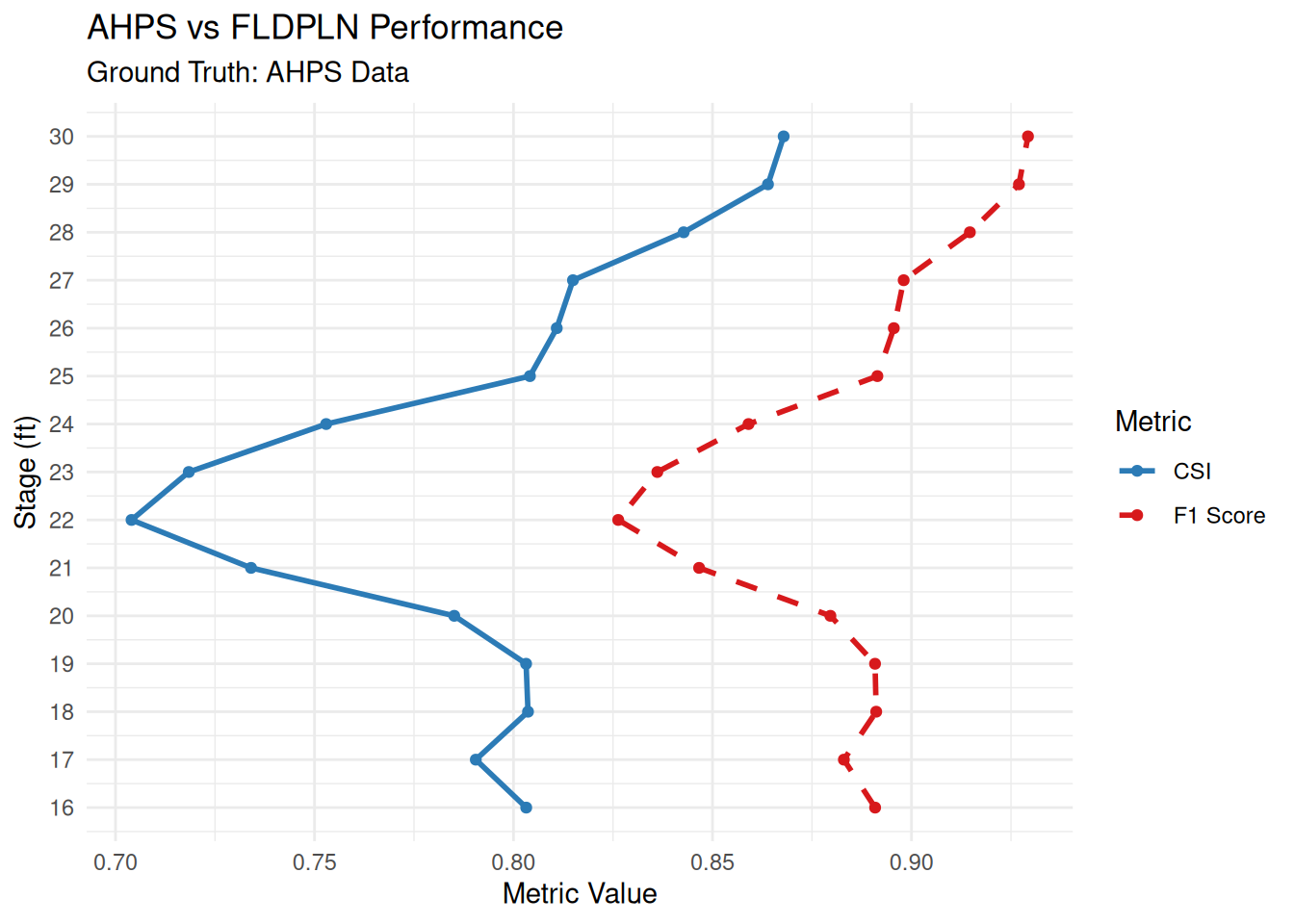
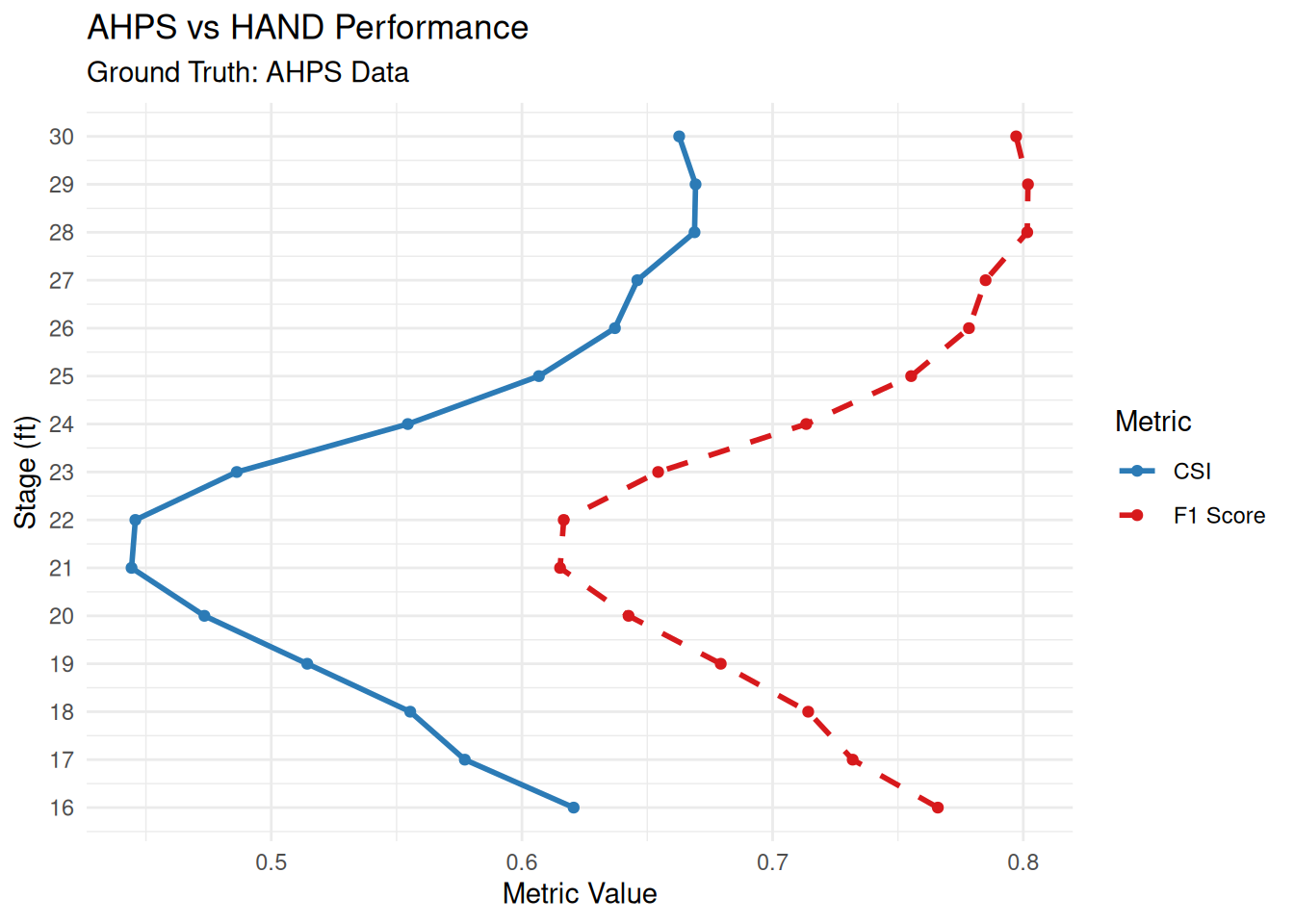
Comparisons using the gauge read stages are quantified across the range of elevations present in the library and plotted in Figure 18 (FLDPLN) and Figure 19 (HAND).

Figure 18: Stage-based performance metrics (CSI and F1 Score) evaluated across river stages for FLDPLN CatFIM compared to AHPS Partner FIM ground truth under direct numerical access.

Figure 19: Stage-based performance metrics (CSI and F1 Score) evaluated across river stages for HAND FIM4 compared to AHPS Partner FIM ground truth under direct numerical access.

Mapped stage access

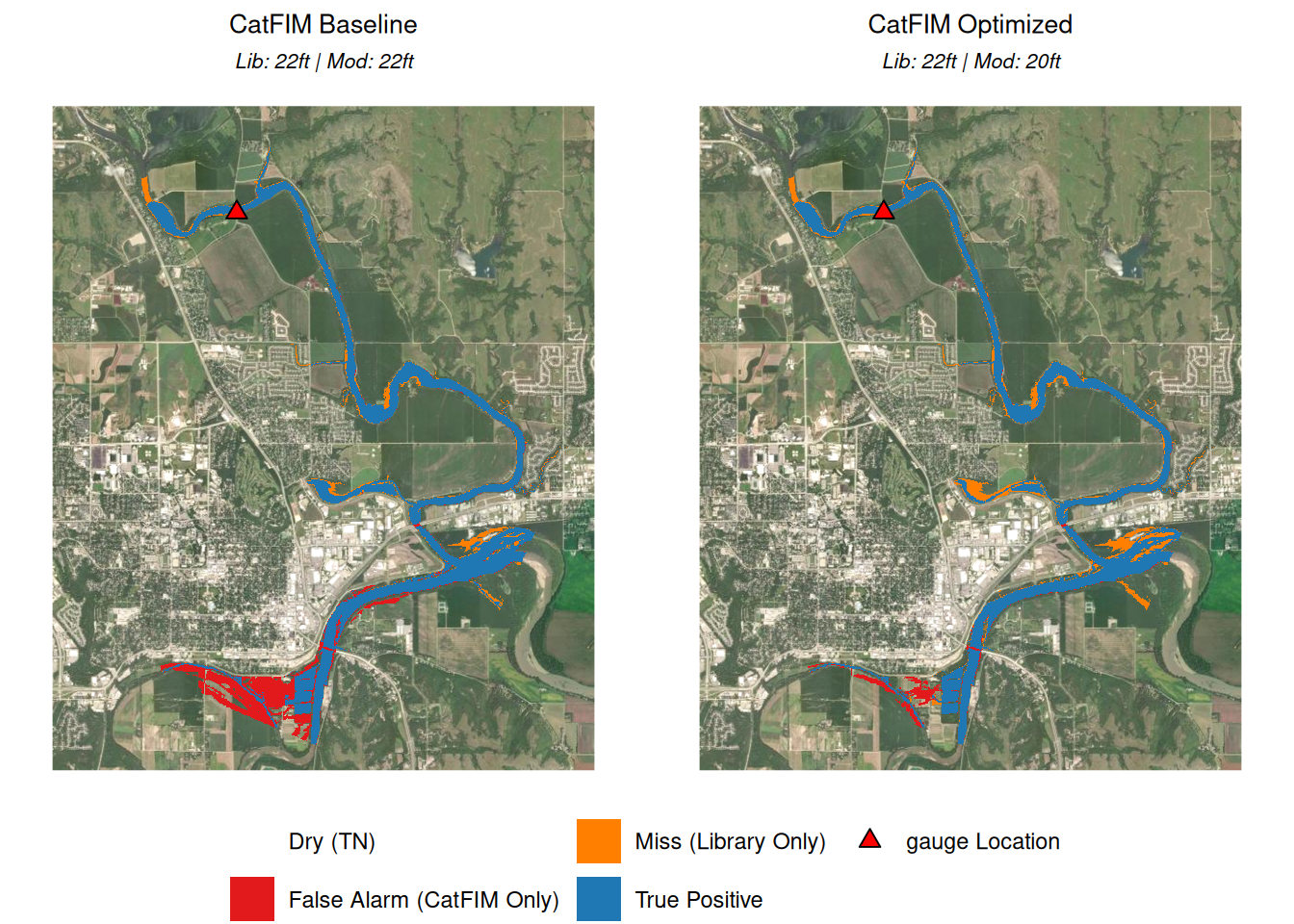
Figure 20 illustrates the spatial distribution of the confusion matrix for the FLDPLN CatFIM under two access patterns (left: direct access; right: optimized library slice). Figure 21 displays the corresponding comparison for the HAND categories.

Figure 20: Spatial confusion matrix comparison between direct numerical stage access (left) and optimized mapped stage access (right) for FLDPLN CatFIM using AHPS Partner FIM as reference.

Figure 21: Spatial confusion matrix comparison between direct numerical stage access (left) and optimized mapped stage access (right) for HAND CatFIM using AHPS Partner FIM as reference.

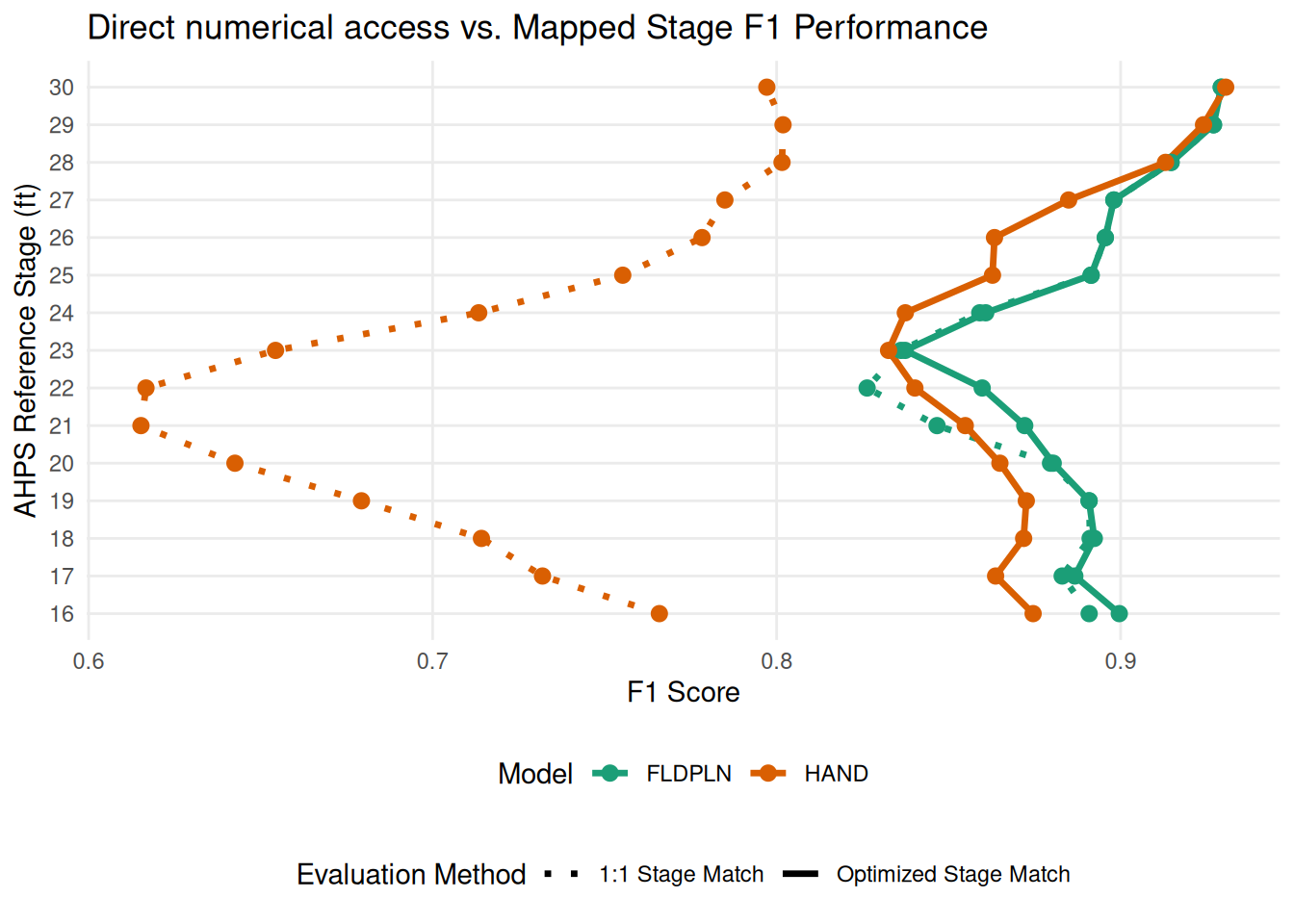
Finally, we compare the improvements to accuracy these different approaches add across the full range of shared values in Figure 22

Figure 22: A full domain comparison of the reported metrics for both categorical FIMS and access patterns.

Discussion

Using the direct mapping of stages resulted in CSI scores for the HAND method that were far below (roughly 0.2 lower) those of the FLDPLN baseline for the same access pattern across the entire range of library stages. Some of these deviations can be explained by intentional differences in how the modeling surface is used. For instance, HAND masks out leveed areas for operational deployment and extends far above the established maximums of the other categorical inundation libraries. This contrasts with FLDPLN, which interpolates stage locally while holding volume constant, allowing it to capture near-gauge references more closely without the broad terrain assumptions made by HAND.

However, when correcting for the access pattern to better capture the reference both models, and the HAND library in particular, see significant improvements in representation. This highlights a critical issue of equifinality in flood inundation modeling: by strictly coupling the concerns of spatial mapping to hydrologic modeling, we often obscure the true spatial skill of a map and hide the cascading uncertainties of other work streams. When a map is accessed based solely on a direct numerical output that contains its own structural biases (such as rating curve errors), the map itself is incorrectly penalized for hydrologic errors rather than spatial inaccuracies. By adjusting the access pattern we can bridge the gap between differing underlying assumptions and extract a more accurate representation of the inundation extent.

This case study demonstrates that with an informed but simplistic offset correction, libraries that might historically be dismissed as unskillful or erroneous can still be highly valuable and informative. This is especially true for areas that lack the deep investments of time and expertise required for customized flood map creation.

However, it is critical to acknowledge the limitations of this single-site comparison. While the application of an optimized mapped stage access pattern dramatically improved spatial representation for the MNTK1 domain, the specific numerical offsets calculated here (e.g., subtracting four to eight feet from the HAND library to match the AHPS reference) are highly localized. They correct for the specific datum assumptions, channel geometries, and rating curve structures unique to this specific river reach. Consequently, these specific numeric offsets cannot be universally extrapolated to other basins across the contiguous United States, where topography and model parameterization vary wildly. Instead, this exercise serves as a methodological proof-of-concept. It proves that a framework of dynamically adjusting the access pattern can recover significant spatial validity from models that might otherwise appear unskillful, rather than providing a universal calibration key.

Conclusions

This validation highlights that while terrain-based models like HAND offer a scalable alternative to detailed, hydraulic-based FIMs, systematic biases remain a challenge. However, this study proves that these structural biases do not render the models operationally useless; rather, they emphasize the need to shift our focus toward how we access and deploy these predictions. By decoupling the hydrologic stage assignment from the underlying spatial map, we demonstrated that optimizing the access pattern can recover significant spatial accuracy that would otherwise be masked by standard, direct numerical evaluations.

We still have a significant amount of work to do before we have fully closed the gap between predicting the flux of water across the landscape and placing a reliable flood map into the hands of a decision-maker. Future efforts to make hydrologic simulations more seamless, flood maps more accurate, and communication more engaging will all contribute to reducing the time and effort needed to make this system more replicable and a little less wicked. Moving forward, standard accuracy assessments and operational deployments must account for these access methodologies. By integrating flexible, optimized access patterns, we ensure that inherently skillful spatial data is not incorrectly discarded due to hydrologic routing or rating curve errors, ultimately providing a more accurate and reliable reflection of reality for end-users.

Chapter 6: Conclusions

This dissertation addresses the systemic “technical friction” that historically isolated localized hydraulic engineering from national-scale geospatial forecasting. Bridging reach-scale hydraulic modeling to a National Water Model framework requires more than increased computing power; it demands a paradigm shift in how model data is stored, processed, and communicated. In Chapter 2, the development of RRASSLER demonstrated that legacy HEC-RAS data still holds substantial value for flood inundation modeling at the national scale and can be made more accessible and reusable. By “spatializing” these models and anchoring them to a common hydrofabric, we extended and enhanced the findability and interoperability of HEC-RAS data for operational deployments. In Chapter 3, we introduced RAS2FIM, a framework that extends engineering-scale hydraulic models and makes them amenable to automated deployments within a national flood modeling framework. In Chapter 4, we quantified the loss in accuracy caused by moving from the initial hydraulic scale to the National Water Model scale. We found that downstream boundary conditions significantly impact the generated operational flood library relative to the hydraulics represented in the larger model. In Chapter 5, we showed that flood map accuracy is a function of the access pattern used, rather than merely a library-to-library aggregation, demonstrating that intentional map access patterns can improve statistical scores.

While the tools and frameworks developed in this work successfully bridge critical gaps in the forecasting pipeline, flood inundation modeling remains an evolving challenge. Moving forward, the hydrologic and hydraulic modeling communities must continue advancing our collective capabilities. A vital next step in this evolution is the standardization of data readers across the broader computational disciplines. By establishing universal conventions for representing hydraulic and hydrologic data, we can drastically reduce the technical overhead required to translate engineering models into larger frameworks.

Coupled with this standardization, future forecast systems and map generation suites must be technically accessible. The automation demonstrated in RAS2FIM shows what is computationally possible, but transitioning these workflows into regular operation requires intuitive environments that do not demand a deep background in hydroinformatics. Lowering this technical barrier will empower local agencies, stakeholders, and practitioners to generate, validate, and deploy their own libraries within a unified national system, thereby contributing to a shared operating picture.

To support these systems and improve the underlying fidelity of hybrid, ensemble-based models, the integration of foundational data and real-time observations must be prioritized. The structural biases and equifinality issues identified in this research are often a direct symptom of data scarcity. Expanding our network of ground-truth measurements will provide future forecast systems with the information necessary to dynamically adjust access patterns based on localized conditions, helping to mitigate the boundary and scale errors observed during national-level conflation.

Ultimately, the value of any flood inundation model is measured by its utility in decision-making. Shifting the focus from merely generating more maps to delivering the right map requires much deeper engagement with end users. Bringing emergency managers, urban planners, and the public directly into the development loop ensures that technical advancements translate into actionable, operationally relevant intelligence. Continuing to reduce the technical friction between hydrologic modeling and spatial mapping will make these systems more reliable, more replicable, and significantly more useful during flood events.

References

Afshari, S., Tavakoly, A. A., Rajib, M. A., Zheng, X., Follum, M. L., Omranian, E., & Fekete, B. M. (2018). Comparison of new generation low-complexity flood inundation mapping tools with a hydrodynamic model. Journal of Hydrology, 556, 539–556. https://doi.org/10.1016/j.jhydrol.2017.11.036

Aristizabal, F., Chegini, T., Petrochenkov, G., Salas, F. R., & Judge, J. (2023). Effects of High-Quality Elevation Data and Explanatory Variables on the Accuracy of Flood Inundation Mapping via Height Above Nearest Drainage [Preprint]. Rivers and Lakes/Modelling approaches. https://doi.org/10.5194/egusphere-2023-1205

Baruah, A., Dhital, S., Cohen, S., Nhan, T., Tran, D., Elhaddad, H., Watts, C. L., Devi, D., Chen, Y., & Pruitt, C. (2025). FIMserv v.1.0: A Tool for Streamlining Flood Inundation Mapping (FIM) Using the United States Operational Hydrological Forecasting Framework. Environmental Modelling & Software. https://doi.org/10.22541/essoar.173991613.37443127/v1

Bhatt, C. M., Rao, G. S., Diwakar, P. G., & Dadhwal, V. K. (2017). Development of flood inundation extent libraries over a range of potential flood levels: A practical framework for quick flood response. Geomatics, Natural Hazards and Risk, 8(2), 384–401. https://doi.org/10.1080/19475705.2016.1220025

Blodgett, D., Johnson, J. M., Sondheim, M., Wieczorek, M., & Frazier, N. (2021). Mainstems: A logical data model implementing mainstem and drainage basin feature types based on WaterML2 Part 3: HY Features concepts. Environmental Modelling & Software, 135, 104927. https://doi.org/10.1016/j.envsoft.2020.104927

Edwards, J., Gomez, F. J., Do, S. K., Weiss, D. A., Kastens, J., Cohen, S., Moradkhani, H., Lakshmi, V., & Li, X. (2025). FLDSensing: Remote Sensing Flood Inundation Mapping with FLDPLN. Remote Sensing, 17(19), 3362. https://doi.org/10.3390/rs17193362

Frame, J. M., Nair, T., Sunkara, V., Popien, P., Chakrabarti, S., Anderson, T., Leach, N. R., Doyle, C., Thomas, M., & Tellman, B. (2024). Rapid Inundation Mapping Using the US National Water Model, Satellite Observations, and a Convolutional Neural Network. Geophysical Research Letters, 51(17), e2024GL109424. https://doi.org/10.1029/2024GL109424

Ghanghas, A., Dey, S., & Merwade, V. (2022). Evaluating the reliability of synthetic rating curves for continental scale flood mapping. Journal of Hydrology, 606, 127470. https://doi.org/10.1016/j.jhydrol.2022.127470

Jafarzadegan, K., & Merwade, V. (2019). Probabilistic floodplain mapping using HAND-based statistical approach. Geomorphology, 324, 48–61. https://doi.org/10.1016/j.geomorph.2018.09.024

Kastens, J. H. (2008). Some New Developments on Two Separate Topics: Statistical Cross Validation and Floodplain Mapping [PhD thesis]. University of Kansas.

Maidment, D. R. (2017). Conceptual framework for the national flood interoperability experiment. JAWRA Journal of the American Water Resources Association, 53(2), 245–257. https://doi.org/10.1111/1752-1688.12474

Nikrou, P., Seyvani, S., Cohen, S., Gangrade, S., Gutenson, J. L., Tian, D., Baruah, A., Follum, M. L., & Kao, S.-C. (2026). Intercomparison of flood inundation models across land use types and hydrological flood stages. Journal of Hydrology, 673, 135410. https://doi.org/10.1016/j.jhydrol.2026.135410

Nobre, A. D., Cuartas, L. A., Hodnett, M., Rennó, C. D., Rodrigues, G., Silveira, A., Waterloo, M., & Saleska, S. (2011). Height Above the Nearest Drainage – a hydrologically relevant new terrain model. Journal of Hydrology, 404(1-2), 13–29. https://doi.org/10.1016/j.jhydrol.2011.03.051

Rebolho, C., Andréassian, V., & Le Moine, N. (2018). Inundation mapping based on reach-scale effective geometry. Hydrology and Earth System Sciences, 22(11), 5967–5985. https://doi.org/10.5194/hess-22-5967-2018

Rennó, C. D., Nobre, A. D., Cuartas, L. A., Soares, J. V., Hodnett, M. G., Tomasella, J., & Waterloo, M. J. (2008). HAND, a new terrain descriptor using SRTM-DEM: Mapping terra-firme rainforest environments in amazonia. Remote Sensing of Environment, 112(9), 3469–3481. https://doi.org/10.1016/j.rse.2008.03.018

Schumann, G. J.-P., Neal, J. C., Voisin, N., Andreadis, K. M., Pappenberger, F., Phanthuwongpakdee, N., Hall, A. C., & Bates, P. D. (2013). A first large-scale flood inundation forecasting model: Large-Scale Flood Inundation Forecasting. Water Resources Research, 49(10), 6248–6257. https://doi.org/10.1002/wrcr.20521

Scriven, B. W. G., McGrath, H., & Stefanakis, E. (2021). GIS derived synthetic rating curves and HAND model to support on-the-fly flood mapping. Natural Hazards, 109(2), 1629–1653. https://doi.org/10.1007/s11069-021-04892-6

Wallace, D. S. (2022). Flood Decision Support Toolbox Executive Summary and Submittal Guidance.

Wilkinson, M. D., Dumontier, M., Aalbersberg, Ij. J., Appleton, G., Axton, M., Baak, A., Blomberg, N., Boiten, J.-W., Da Silva Santos, L. B., Bourne, P. E., Bouwman, J., Brookes, A. J., Clark, T., Crosas, M., Dillo, I., Dumon, O., Edmunds, S., Evelo, C. T., Finkers, R., … Mons, B. (2016). The FAIR Guiding Principles for scientific data management and stewardship. Scientific Data, 3(1), 160018. https://doi.org/10.1038/sdata.2016.18

Footnotes

1. largely inflicted by the longboard