CoastalFlood

CoastalFlood generation

One of the more authoritative coastal FIM libraries is the Eastern Region Headquarters CoastalFlood page (recreated above). This service presents flood extent libraries derived from a MHHW datum and the impacts based on classifications from NWS impact statements (Flood Extent, Moderate Extent, Major Extent); plus an Major Extent +1 foot of elevation, Major Extent +2 feet of elevation, and Major Extent +3 feet of elevation added. These services can be loaded in from their rest service, but because the methodology is accessible it’s an instructive exercise in both dataset acquisition and interpolation to replicate these libraries.

Background

The CoastalFlood product is generated by generating a MHHW datum from a set of gages. This process is covered in extensive detail in Sweet et al. (2018), and we can take those values from our gage network. The CoastalFlood product covers primarily the domain of the Atlantic ocean seaboard, and this is certainly where the greatest density of gages are.

We’ll start with the topobathy from Lynker Spatial (you can pull those from here

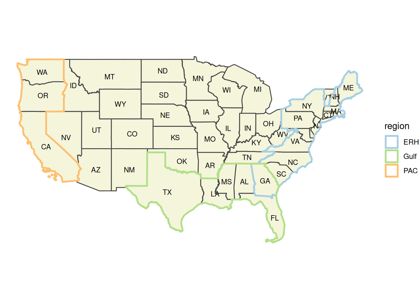
To make this problem more computationally tractable, we’ll break the domain up into several larger constituent zones; the Atlantic seaboard covering the states taht the coastalFlood product covers (ERH), the rest of what falls into the Atlantic domain, including Florida and the Gulf states (ATL), and the Pacific seaboard (PAC).

The first step is to establish that MHHW datum. While we can transfom virtually any point using vadtum, the CoastalFlood surfaces in particular are generated by applying the datum correction specifically at gages and then interpolating between them. The impact stages are fortunately a default field in the provided gage files and so we don’t need to do any extra manipulation to gather those. Our workflow to generate those surfaces will look like so:

CoastalFlood workflow

flowchart TD
    %% Node Definitions
    AHPS[(NWPS Obs & FCST)]
    
    subgraph A[CoastalFlood Method]
        direction TB
        COOP_THR[(COOP derived inundation spreadsheet)]
        COOP_MHHW[(MHHW interpolation)]
        COOP_SURF[(Inundation threshold surfaces)] 
        COOP_MASK[(Drop Land/Land and Water/Water classes)] 
        COOP_DEL[(ESRI tile service .tpk for AGOL)] 
    end

    prototype[prototype.html]

    %% Connections
    AHPS ==> COOP_MHHW
    COOP_MASK ==> prototype

    %% COOP Path Flow
    COOP_THR ==> COOP_MHHW
    COOP_MHHW ==> COOP_SURF
    COOP_SURF ==> COOP_MASK
    COOP_MASK ==> COOP_DEL

    %% Classes
    classDef output fill:#f9f,stroke:#333,stroke-width:2px;
    class OWP_DEL output;

Let’s make this toy example a tiny bit nicer, we’ll focus in on only a few of the New England states. The first step is to establish that MHHW datum. We’ll do this by identifying the gage datum elevation, and using the operational gage network to back our way into a MHHW datum. It’s worth noting that this is not the MHHW datum, but a MHHW datum derived from an operational scraping of the gages. The more methodologically robust approach would involve reprojecting these with vdatum transformation to backing out these elevations but for the scale and objectives of this application, this assumption is fine. Once we’ve narrowed out our gages, these look like so:

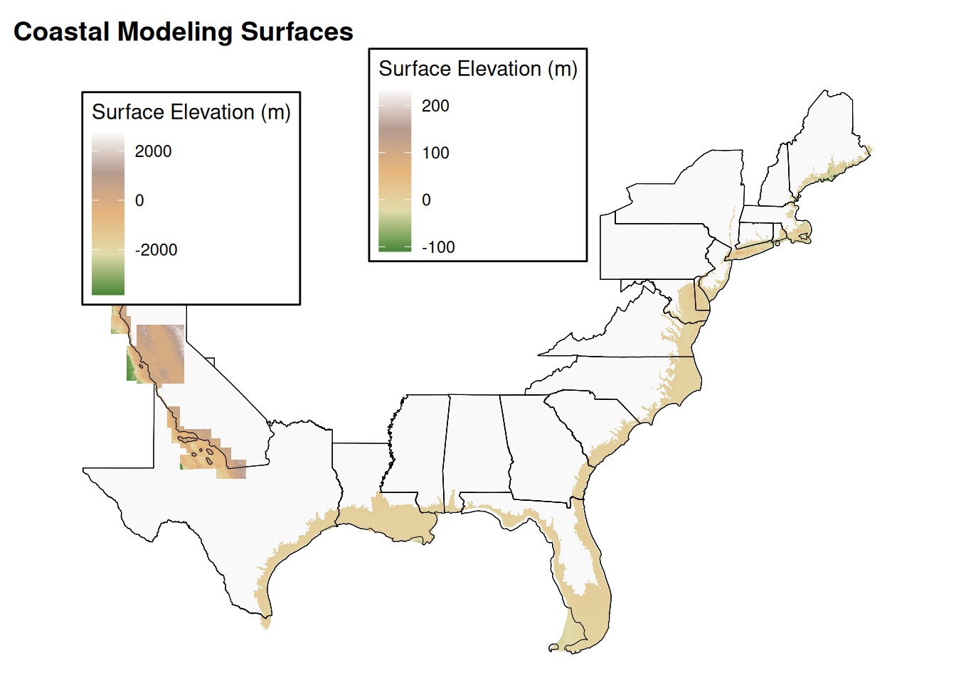
Then we’ll construct a navd88<>MHHW 0 surface by taking our gage datums and correcting them for the MHHW observations that come from our network.

Because these are now local surfaces to us, we can view them like so:

Finally, let’s throw these into a mirrored viewer to gain an appreciation for how much we’ve deviated from that far more authoritative NWS surface.

References

Sweet, William, Greg Dusek, Jayantha Obeysekera, and John J. Marra. 2018. “Patterns and Projections of High Tide Flooding Along the U.S. Coastline Using a Common Impact Threshold.” NOAA Technical Report, ahead of print, February. https://doi.org/10.7289/V5/TR-NOS-COOPS-086.