Lab 09B - Cloud based GIS

This lab is ungracefully ripped from my own tutorial on the UCGIS BoK entry for GEE. Please explore this version for more information and background.

Google Earth Engine is still a beta product, and you will need to request access to the platform through your Google account here. These are still approved by hand and may take a few days to get. Once approved, you will need to follow the instructions in the email that is sent before you are able to access the platform. Therefore, be sure to do this step before you attempt to work though this lab.

This lab serves as a highly hand held introduction to Google Earth Engine and cloud based geospatial operations. There will be a lot of code to look at here, but no prerequisite code experience is necessary and the steps have been broken into small, digestible pieces. The goal by the end of this tutorial is not that you have become an expert in JavaScript, but that you see the power and potential that cloud based geospatial analyses offers, and that you come away with a deeper appreciation for the technology necessary to facilitate effective global scale operations.

Outline:

You are submitting a URL to blackboard. There are no questions to answer or

Snow cover frequency, or the number of days that a spot is covered by snow divided by the number of days it has a valid observation, is an important metric of the cryosphere, and is critical to a number of biogeophysical processes. Using the daily MODIS snow cover dataset, we will calculate the snow cover frequency on a yearly basis for water years 2003 through 2018. A water year here is defined as October 1st to September 30th and is labeled as the year of the end date. For example, water year 2004 is from Oct. 1, 2003 to Sept. 30, 2004. We will then find and map the linear trend of snow cover frequency at every pixel across the globe. To add a little more nuance on this analysis, we will take into account the sensor zenith angle of each MODIS observation. At the extremes of the MODIS instruments sensor zenith, the pixel length has essentially doubled, and the width has increased more than 10 times that of the nidar pixel. These observations can skew aerial coverages, so we want to limit our daily snow cover dataset to just those observations that have a sensor zenith angle less than 25o, limiting pixels to 110% of the nominal area of a nadir pixel. To do this we need two daily datasets, the daily snow cover product MOD10A1 and the sensor properties contained in the MOD09GA dataset, both are available in GEE.

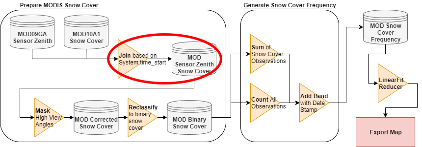
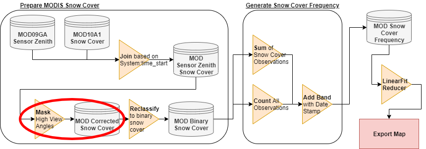
To accomplish this analysis, we will first need to join the two datasets (MOD10A1 and MOD09GA), to create a combined dataset. We then need to mask out those pixels with a high sensor zenith angle. After that, we need to reclassify the snow cover to a simple snow/no snow/missing dataset, which will make future calculations easier. After reclassifying the data, we want to count at each pixel the number of days that have a snow observation and the number of days that have a valid observation. We will then need to add a band representing the water year (time) and calculate the trend at each pixel before finally exporting our results. The steps of this process are exemplified in Figure 3. We will wrap much of that data up into functions, as outlined below, in the larger ovals. The general process we will follow is shown in Figure 3.

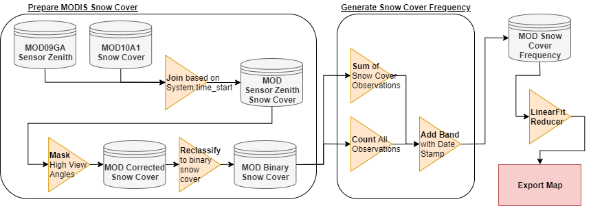
A schematic of data analysis flow.

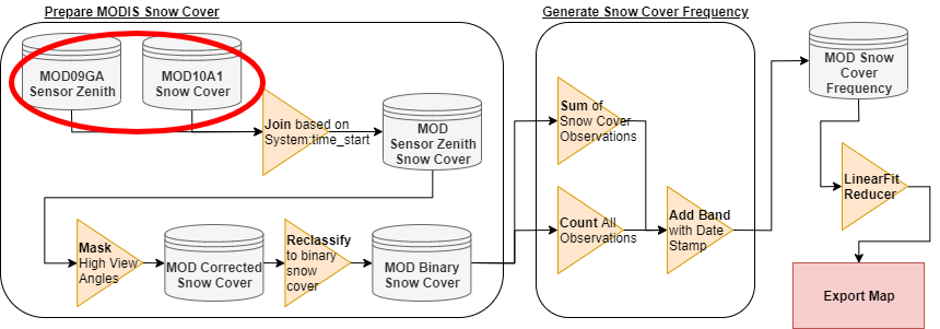
Where we are in relation to the rest of our analysis. Here we explore the data and learn its associated structure in GEE.

Looking at Figure 4, we will start by accessing the MOD10A1 dataset and examine its structure. You can search for the datasets with the search bar at the top of the Code Editor, and use associated GEE data IDs to access them. We start by searching for MOD10A1, and importing it, as shown in Figure 5. Using just over 40 characters, we have access to the entire MOD10A1 dataset in less than 20 seconds. These static variables can also be included as Imports, which sit above the code editor as Imports.

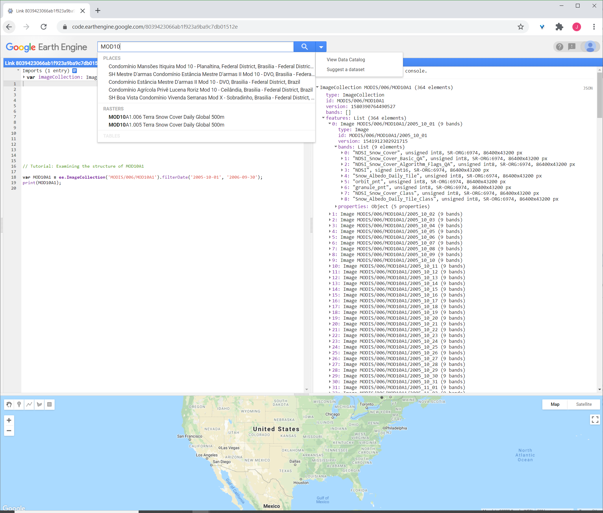
The view of the Code Editor IDE and how to import an ImageCollection into the API for analysis. The code is available at https://code.earthengine.google.com/8039423066ab1f923a9ba9c7db01512e

We can see that MOD10A1 is imported into your JavaScript as an ImageCollection. If you recall, the MOD10A1.006 data product is a daily global snow cover dataset and each Image in the ImageCollection has 9 bands. The one we are interested is the “NDSI_Snow_Cover” band which is a fractional snow coverage band with valid values from 0-100. Although the quality band has a high sensor zenith flag, the full sensor zenith angle data is only found in the MOD09GA.006 dataset. Therefore, our next goal is to join the two datasets together.

Where we are in relation to the rest of our analysis. Here we demonstrate how to join collections.

After we import the MOD09GA dataset as another ImageCollection, our goal is to get the sensor zenith angle band from the MOD09GA ImageCollection to join with our snow cover data. To select a particular band to work with, we can use the .select() method, as shown in Figure 7.

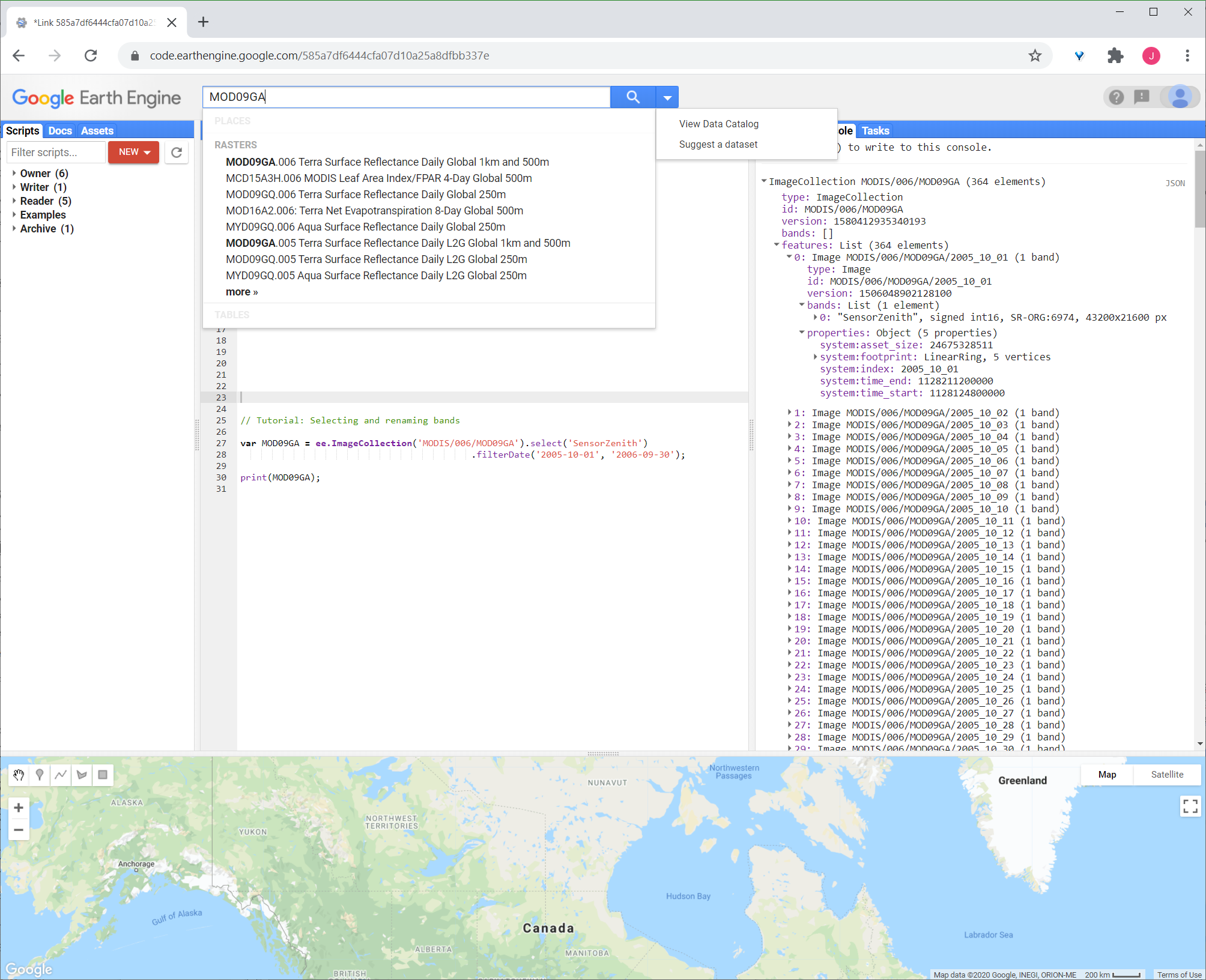
Example of using the .select() and .filterDate() methods in GEE to pull images we need and examine their structure. The code is available at https://code.earthengine.google.com/585a7df6444cfa07d10a25a8dfbb337e

Joining two collections requires a common property between them, just as it does in standard GIS software. In this case the best way to go about joining the collections is to join them based on their acquisition times, using the “system:Time_Start” property as the filter. If you look at the various types of joins in the documentation, you will see that there are a few ways to do this but we will use the join.inner(). The code to join the two datasets together is shown in Figure 8.

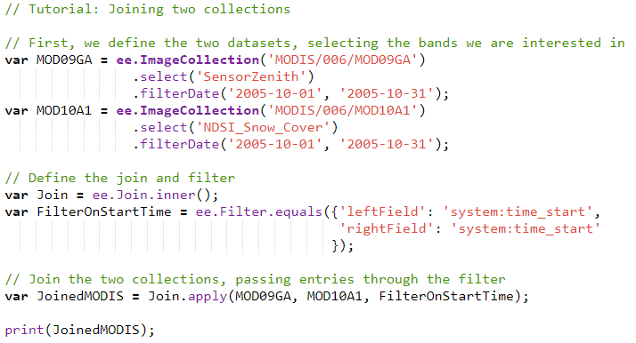
The code used to join the two MODIS datasets together, which is available at https://code.earthengine.google.com/e63a22be50d2c017363d22d0d0d1c423

We’ve just joined two MODIS collections together, and it took less than 20 lines of code to do so! However, if you print the resulting collection you will get something that looks like Figure 9.

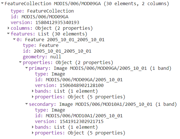
Printed results of the joined collection, itself the result of the previous code execution.

The output collection from the join operation is a FeatureCollection, where the matching images are the “primary” and “secondary” properties of the features. In order to convert this to a format that we can work with, we need to run a function across the FeatureCollection, creating a new image that has the bands from the primary and secondary images. You can visualize the conversion as a series of operations shown in Figure 10.

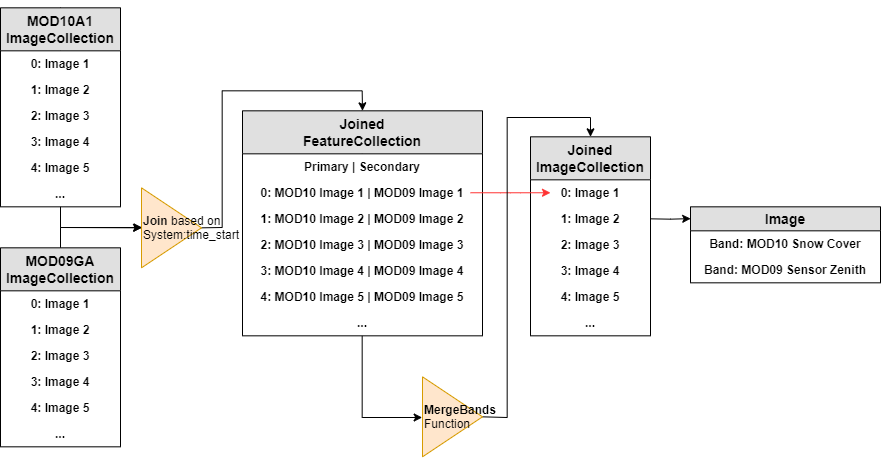
The schematic of the MergeBands function we need to write to transform the results of our join into a more useable form.

The code for the MergeBands function and for applying the function to each matching pair of images in the FeatureCollection are shown in Figure 11. When run the code, be sure to note the difference between the input and output collections.

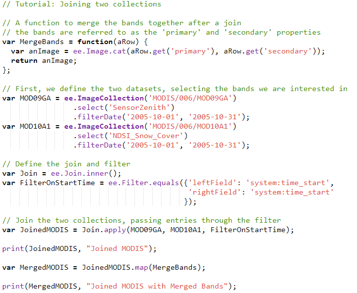
The code (available at https://code.earthengine.google.com/81bac4a77cf20821f86ad94b7611d457) for the MergeBands function and for applying the function to each pair of matched images, which convert the joined collection to a form more useful for subsequent analyses

Now that we have joined the two collections, we need to remove the pixels that have a sensor zenith angle greater than 25o.

Where we are in relation to the rest of our analysis. Here we demonstrate two useful functions to create a sensor filtered dataset.

As shown in Figure 12, with snow cover and zenith angle joined into images as bands, we need to remove the pixels from each image that have a sensor zenith angle larger than 2500 (the angle is stored as a multiple of *100). To do this we will introduce two of the most useful functions in GEE, .map() and .mask(). As seen in the MergeBands function, we used the .map() method. This method executes the same function across each element in a collection, and returns a collection of the same depth. Masking is another helpful method we’ll use. The input of mask is applied to the image and anything which isn’t specified within is converted to a null value. Figure 13 shows a simplistic example where we use the .mask() method to keep only the areas with an elevation larger than 2000 m from the SRTM90 elevation dataset in the image.

The code (available at: https://code.earthengine.google.com/60187ddb4b541fb209697f2c6820c65d) and results of an example .mask() method.

Using the .mask() and .map() methods, we’ll modify our code to mask out any pixels with a sensor zenith angle greater than 250. Because we want to do this for every image in the ImageCollection we will use the .map() method with the MaskSensorPixels() function as shown in the highlighted portion of Figure 14.

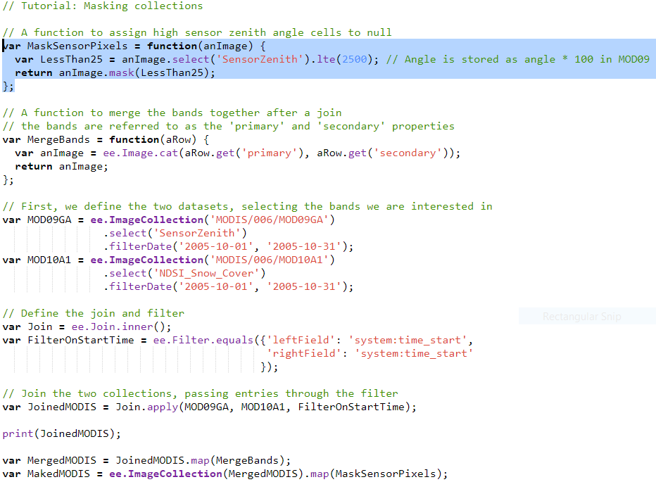
The code for masking out large zenith sensor angle pixels, which is available at https://code.earthengine.google.com/bfed155a968160db67253474cd707c9f

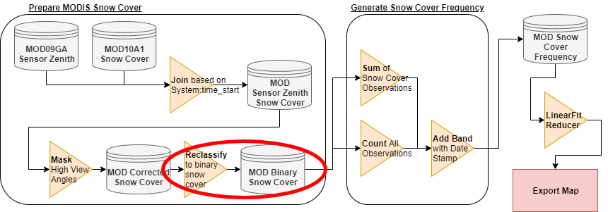
Where we are in relation to the rest of our analysis. Here we need to reclassify our snow band to a binary no snow/snow dataset.

As shown in Figure 15, our next step is to reclassify the pixels on each image to snow, non-snow or missing. The “NDSI_Snow_Cover” band in MOD10A1.006 is a fractional band with valid values from 0-100, indicating the fractional snow coverage at a pixel. To perform a snow cover frequency analysis, we need to reclassify the band into the no-snow/snow/missing categories, using values that represent “snow” as 1, “No snow” as 0, and null for ‘missing’ values. To accomplish this GEE has a remap() method, which takes a list of values and maps the values to another list of values you specify. Because we need to reclassify every image in the collection, we will use the handy .map() method again. We are now at the end of our first data processing chain, “Prepare MODIS Snow cover”, meaning we can wrap up all the previous steps into a single function, PrepareModisSnowCover(), that takes two dates, a StartDate and a StopDate. The code to do this is shown in Figure 16. As an aside, these last few steps could be wrapped up in the same .map() call, but were separated here for demonstration purposes.

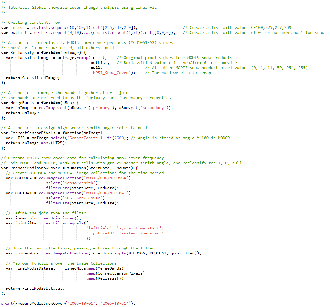
The code used to generate a year of sensor-zenith-angle filtered, reclassified snow cover data, available at https://code.earthengine.google.com/5e68e31ee7ead90a6d33b80ab8826e55

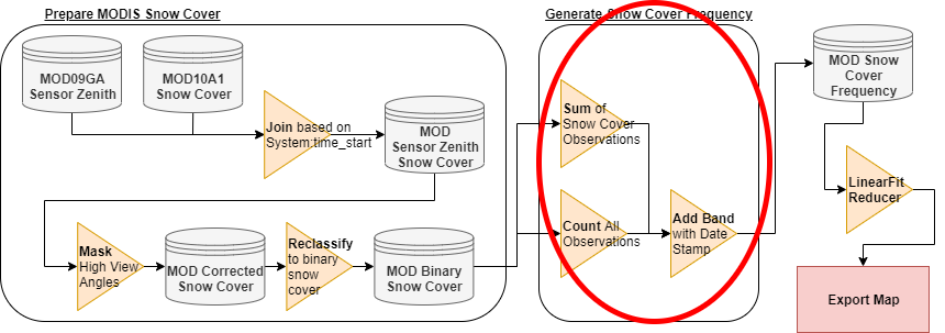
Where we are in relation to the rest of our analysis. Here we need to create a function that generates a time series of images which stores the snow cover frequency and the date of the image.

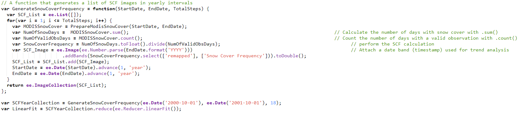
Now that we have a function to create a processed MODIS snow cover dataset for a given time interval we need to construct a function to generate a time series of snow cover frequency as outlined in Figure 17. The PrepareMODISSnowCover function returns a single band, called remapped, that represents a sensor adjusted and reclassified snow cover for each day of the collection. In order to calculate snow cover frequency we need to know both the number of snow days and the number of days we have valid observations. The .count() method in GEE counts the number of times a pixel has a valid value within an image collection, and will ignore (not count) those images that have a null value, so it counts both snow and no-snow values in a pixel stack. We can also count the number of snow days at a pixel by using the .sum() method, which adds the values of a stack of pixels. We will wrap this up in a function that takes a start and end date, and the number of intervals to advance. This code to accomplish this is shown in Figure 18 below:

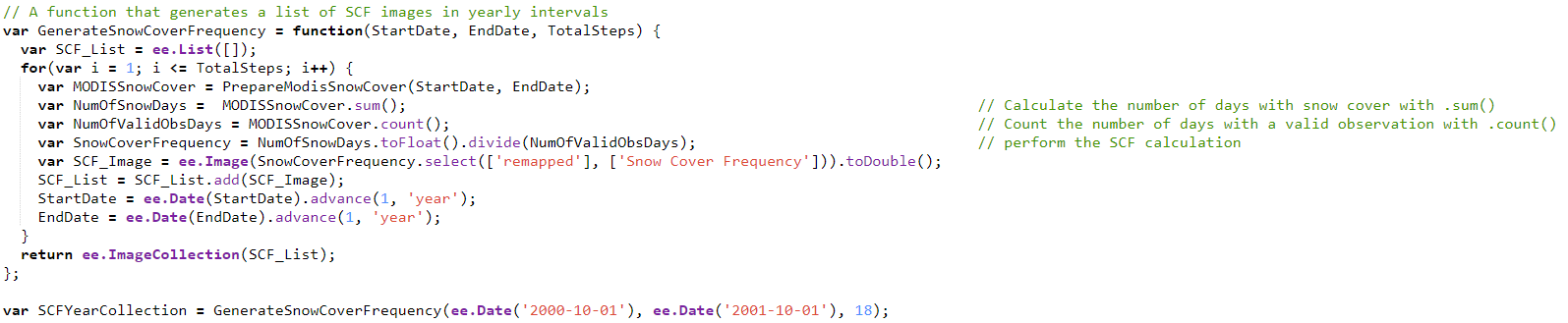
The code which calculates snow cover frequency within a certain time interval is available at https://code.earthengine.google.com/aeee1a828fb717397d38eaef236ed498

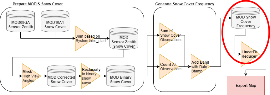
Where we are in relation to the rest of our analysis. Here we need to pass our final dataset to the LinearFit Reducer.

As outlined in Figure 19, we have now created the necessary functions to create a time series of snow cover frequency, but to calculate a linear trend we also need a band which represents the time stamp. With a small modification to the GenerateSnowCoverFrequency, we can add the EndDate as a numerical band, which gives us everything we need to calculate the linear trend. If we look at the documentation, ee.Reducer.linearFit() returns an image with two bands, one called ‘scale’ and one called ‘offset’. This is Google’s terms for ‘slope’ and ‘intercept’, so the value we are after is the scale. The code to do so is shown in Figure 20.

The code to create snow cover frequency and linear trend is available at https://code.earthengine.google.com/c5dd98445765937e9ff1c1f4f6d24ec5

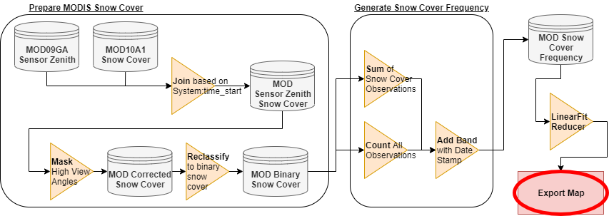
Where we are in relation to the rest of our analysis. Now we need to display and export our analysis.

As we can see from Figure 21, we are at the end of our analysis. The final step is to visualize and export the analysis so that others can view it. The first thing we need is to do is create color palettes. We then filter the slope based on a minimum value of snow cover frequency using the .mask() function with a .min() reducer over the entire collection. This ensures that we are not displaying the trend analyses for areas that have very low snow coverages. We then use the Map.addLayer() method to add a layer to the map, setting the min and max values and the palette we want. Then we will export our analysis as a GeoTIFF using Export.Image.toDrive(). For a little more flair, we’ll also export the timeseries of snow cover frequency as a video using Export.video.toDrive(), using another .map() call to force images into rgb space for video. The code to accomplish this is shown in Figure 22.

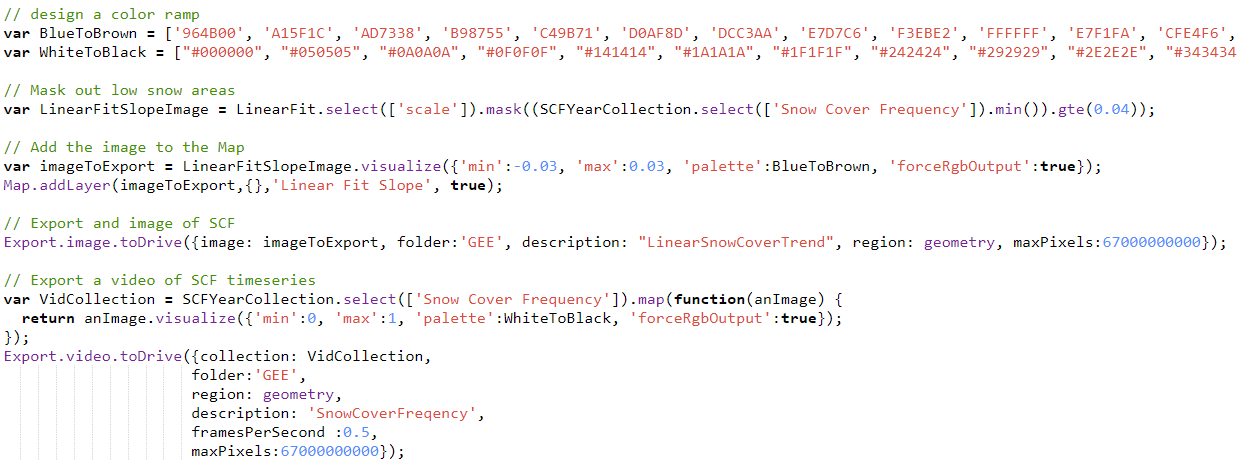
The code to accomplish the display and export of our analysis, available at https://code.earthengine.google.com/3ac848247d0e231e50c5feefd7d23f6d

Finally, let’s capitalize on the advantage of the new UI and app features in GEE to create an interactive web map so that anyone may view our analysis. The UI Examples provide several great frameworks to construct an app, so we will borrow some of them to create an application using our new snow cover trend data. The code to do so look like so: https://code.earthengine.google.com/bc3998bc98afca2007249eff2d8c6a1a. If you publish the app using the app button above the map and following the clicks, anyone can access the analysis at a URL similar to https://JamesMColl.users.earthengine.app/view/bokdemo as shown in Figure 23.

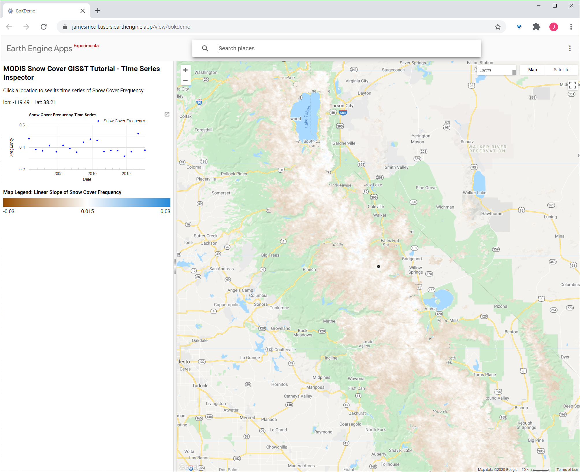
An interactive web application based on this analysis, available at https://JamesMColl.users.earthengine.app/view/bokdemo

Taking a step back to look at what we’ve accomplished in this tutorial really accentuates what can be accomplished using GEE:

• We pulled in 18 years for two daily MODIS datasets
• Joined them in space and time
• Filtered and reclassified the resulting dataset
• Calculated snow cover frequency
• Performed the linear fit with the snow cover frequency dataset
• Exported a GeoTIFF and video of the resulting slope map
• and created a web application so that anyone can interact with the analysis And the entire process probably took less time to perform than it would have needed to download a single day of MODIS data. This is just a small sample of the processing power and capabilities that Google Earth Engine has to offer, and an example of how this platform has revolutionized global scale geospatial analyses.

Taken as a whole, GEE represents the most advanced, cloud-based geoprocessing platform to date. Although several other platforms encompass some of these aspects, no suite of tools currently available can replicate the access to geospatial data, relative simplicity of use, and sheer power of analysis that GEE offers. The platform is constantly under development and new features and algorithms are continuously updated. The GEE team and community is also incredibly approachable and helpful with GEE booths are commonly seen at many geospatial meetings, where they demo use cases and announce new features.

Question to submit
Using the code and app above, do the following.

1. Navigate to someplace interesting in the world. Take a screenshot of the snow cover trend in that area and paste it at the top of your word document.
2. In 1-2 complete paragraphs below that, answer the following:

• describe and interpret the trend and why it interests you.
• Why do you think this trend is occurring? What other information do you think you’d need to fully describe why the snow cover is changing in this way?