Lab 08 - Advanced Terrain Analysis
In this lab we’ll cover a variety of terrain analysis techniques including shelter analysis and a suite of tools within the hydrology toolbox.
Lab 8: Answer Sheet
Name:
Part 1
Question 1:
What is the value of the majority of the cells on the focalcells raster layer?
Where are the cells with smaller values located?
and why do they have smaller values?
Question 2:
What is the value range in the shelter analysis raster layer?
________ to ________
A large positive value means:
A value close to zero means:
A small negative value means:
Question 3:
What is the interpretation of the sinks output? What would the correct symbology of this layer look like?
Question 4:
Paste your final unit hydrograph here.
| Relevant part | Data Name | Description |
|---|---|---|
| Part01 | chase_dem | DEM for Chase County, KS (30m cell size, elevation in feet) |
| Part02 | Pour_point | A point feature layer that depicts the outlet downstream of the Little River where you'll create a unit hydrograph. |
| Part02 | Stowe_boundary | A polygon feature layer that depicts the boundaries of Stowe, Vermont. This layer was derived from data available from [Vermont Center for Geographic Information (VCGI)](https://vcgi.vermont.gov/) |
| Part02 | Stowe_DEM | A raster layer that depicts elevation within the study area. It also has a resolution of 30 meters. It was derived from data made available by the [United States Geological Survey (USGS)](https://www.usgs.gov/). |
| Part02_worked | Stowe hydrology folder | A worked version of part 2 in consideration of processing power |
This lab, and part 2 in particular, can take a while when CPU is a limiting concern. I can offer a few suggestions, and an alternative.
- Pick a smaller area to process.
- You can skip step if you are careful, as outlined in the instructions.
- If you pause drawing that may speed up UI interactions
- When not actively manipulation the tools you can multi-task. Take the time to understand the workflow, fire off a process, and move onto something else. Try not to have anything super intensive running in conjunction, but light Microsoft office work shouldn’t break you.
- As a stopgap if it’s taking too long, I have provided a copy of my part 2 for you to look over. Use this only if needed.
- A great album to jam to while working.

In this part of the lab, we will perform a terrain exposure analysis, referred to as shelter analysis. The outputs of this workflow are quite popular in archeology studies and inform us as to how protected a given location is.

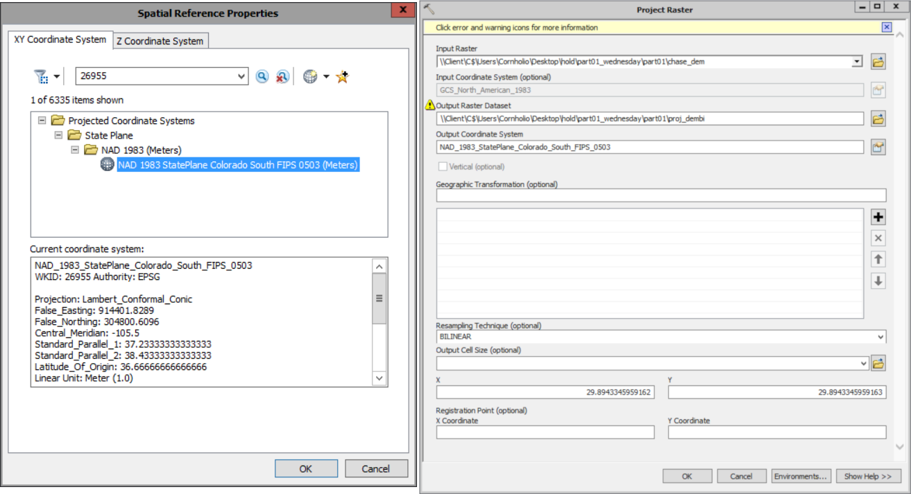
1) Start Arcmap and rename the data frame to Terrain Exposure Analysis. Because we are working at a relatively small geographic scale, we should first reproject our raster from it’s native projection (GSC_North_America_1983) to a more appropriate one for this analysis (NAD_1983_StatePlane_Colorado_South_FIPS_0503 WKID: 26955).
- Open ArcToolbox and navigate to Data Management Tools | Projections and Transformations | Raster | Project Raster
- For your Input raster select you chase_dem from your lab08\part01 folder using the browse button.
- Here we use the browse button to avoid data locks on the elevation data and avoid inadvertently assigning a projection to the dataframe prematurely.
- Call the Output raster proj_dem saved in your lab08\part01 folder
- To select an Output coordinate system, click on the Spatial Reference Properties Button (the hand with the card)
- Define the coordinate system as:
- Projected Coordinate Systems > State Plane > NAD 1983 (meters) > NAD 1983 StatePlane Colorado South FIPS 0503 (meters).prj
- You can also use the search tool to find it, 26955
- Click OK
- Set the Resampling technique to BILINEAR and click OK
2) Finally, convert the elevation from feet to meters.
- Raster calculator expression: proj_dem * 0.3048
- Name the output chase_m
1) First let’s calculate the volume of earth per cell.
- Raster calculator expression, we can round here:
- chase_m * 30 * 30
- Call your output volpercell
2) Finally, use Focal Statistics to calculate the focal sum of this raster layer using a circular neighborhood with a radius of 2 cell size.
- Save the output raster layer as earthvol
1) Create a flat surface using Raster Calculator to create a constant raster layer on which all of the cells have a value of 1.
- (“chase_m” / “chase_m”) will do the trick.
- Make the output raster a permanent raster named constant
2) Use Focal Statistics to calculate the focal sum on the constant raster layer using a circular neighborhood with a radius of 2 cell size.
- Save the output raster layer as focalcells
3) Calculate the earth volume within the circular neighborhood assuming all the cells inside the neighborhood have the same Z value as the focus (“volpercell” * “focalcells”)
- Save the output raster layer as flatearthvol
- Answer question #1 on your assignment sheet
- Calculate the shelter raster layer by subtracting flatearthvol from earthvol
- Save the output raster layer as shelter
After some stylization, you might end up with a map that looks like so:
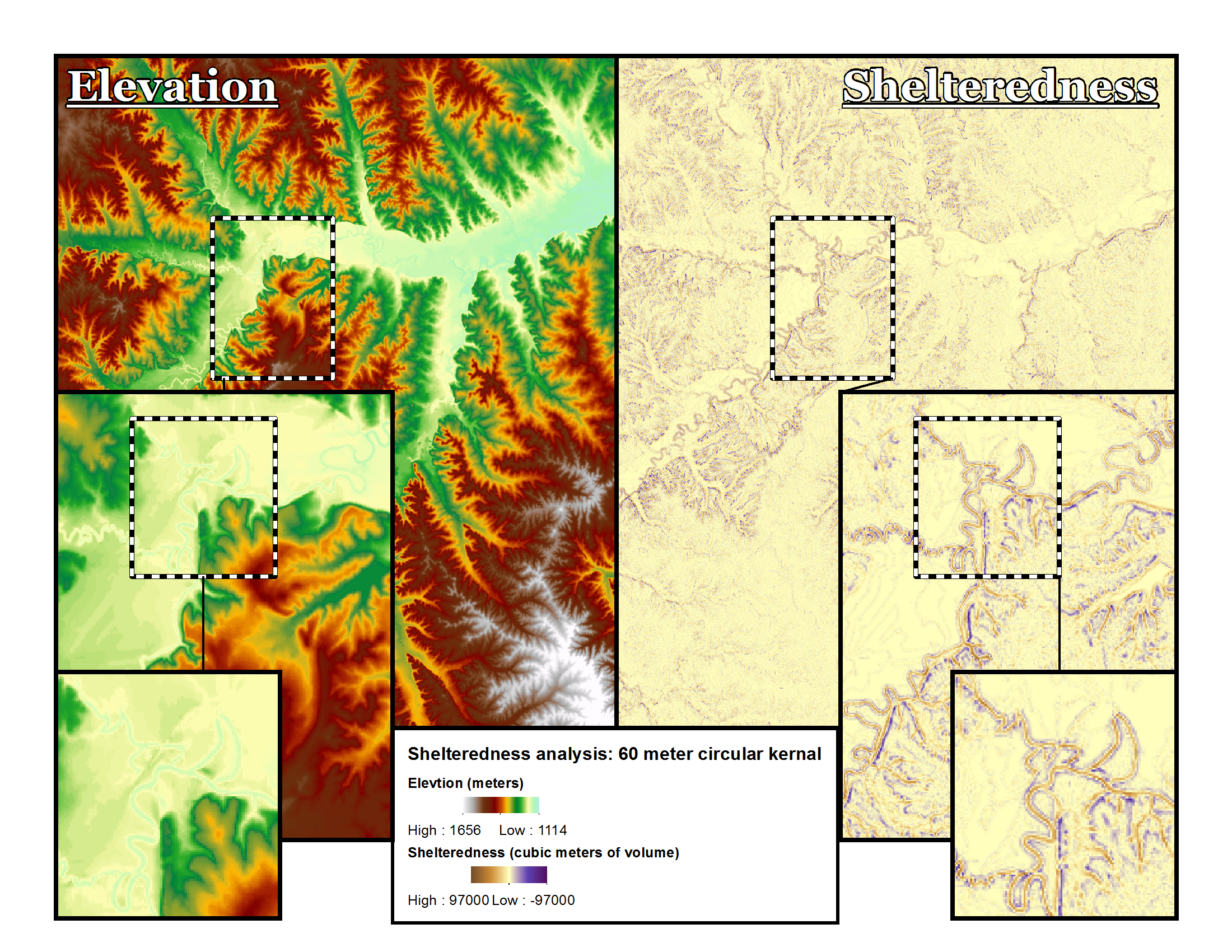
- Answer question #2 on your assignment sheet
The instructions herein are guided by material gratefully pilfered from https://learn.arcgis.com/en/projects/predict-floods-with-unit-hydrographs/
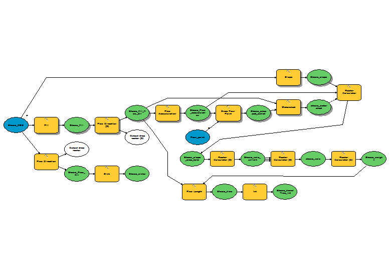
As is the case with many locations across the globe, when disaster strikes planners and residents realize they have data gaps that they can not readily fill. Exampled here, the town of Stowe in Vermont suffered considerably when the remnants of Hurricane Irene stuck the Green Mountain region in August 2011. The Little River overflowed and washed out roads, bridges, and culverts. In an effort to learn more about the event, officials tried to recreate the event using a number of techniques. One way to do this is to construct a hydrograph, which are line graphs determining how much water a stream will discharge during a rainstorm. In this lesson, you’ll create those hydrographs using data provided. If you’re interested in trying this for yourself I encourage you to download and run an area meaningful to you. Refer back to lab 1 if you need a refresher on how to acquire elevation data. The model builder is shown below:
Either import the Stowe_DEM and Pour_point or download and select your own pour point for this analysis.
1) First, you’ll identify sinks in your DEM. Although your DEM was derived from reliable data provided by the USGS, sinks may still be present. In order to identify them we need to know which way the water flows over the surface. The first tool in the workflow is the Flow Direction tool.
- For Input surface raster, choose Stowe_DEM.
- save the output as Stowe_flow_direction in the geodatabase.
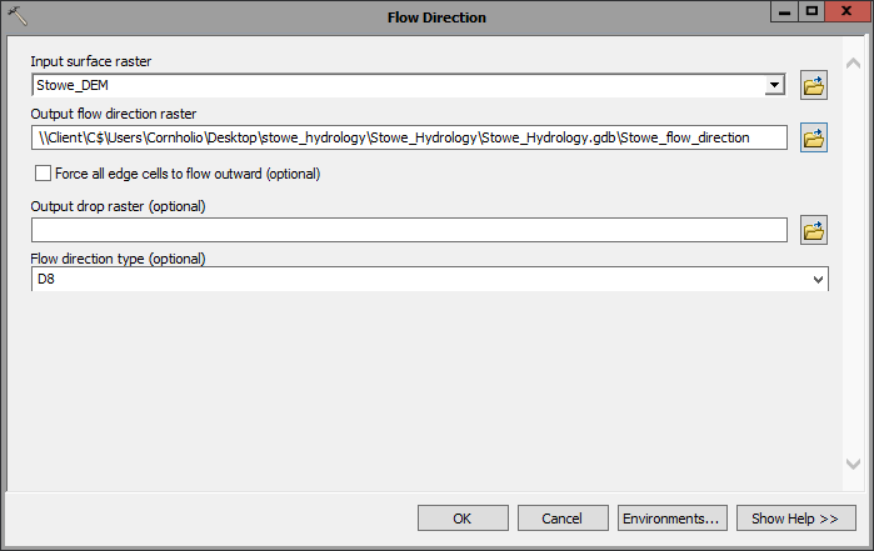
The symbology of the resulting layer corresponds to the direction water is likely to flow. The layer’s appearance isn’t important to this analysis, we just need this layer to run the next step…
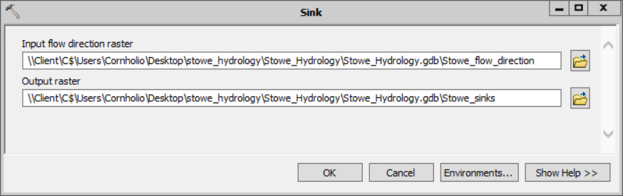
2) Open the sinks tool, the next step in the analysis.
- For Input D8 flow direction raster, choose Stowe_flow_direction.
- Save the output as Stowe_sinks.
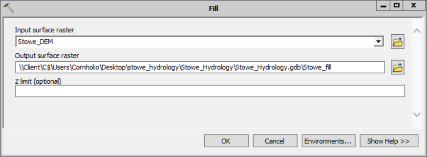
3) The final step in the current task uses the Fill tool to remove sinks from a DEM.
- For Input surface raster, choose Stowe_DEM
- Name the output Stowe_fill.
Having now removed sinks from the DEM, it is considered “hydrologically conditioned” and is ready for hydrological analysis. We’ll use this DEM to determine the watershed area for the outlet point south of Stowe (or wherever you want to drop your point!). A watershed area is the area in which all flowing water will flow toward a certain point—in this case, your outlet. With the watershed area, you’ll be able to limit your subsequent analysis results to the relevant area for your outlet. Determining a watershed requires two components: a flow direction raster layer and an accurate outlet point. One of the most common reasons for a watershed analysis to fail is when the pour point is not adequately aligned to the flow grids. For that reason the Snap Pour Point tool is often included in a workflow. This step can be skipped if you are deliberate with your placement of the point, but I’ll walk through the workflow using it here. First, you’ll determine the stream’s exact location by calculating the areas where water accumulates the most. Then, you’ll snap the outlet point’s location to match the stream and verify it.
The first step to delineate a watershed is to determine the direction that water will flow in your DEM. That way, you can determine the areas where water will flow to the outlet. To do so, you’ll…
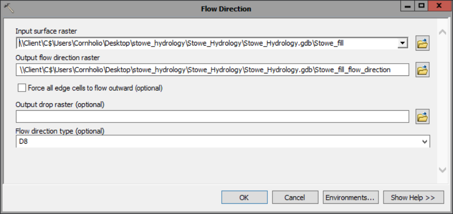
1) Create another flow direction raster layer, this time for your DEM with filled sinks.
- For Input surface raster, choose Stowe_fill.
- Name your output Stowe_fill_flow_direction.
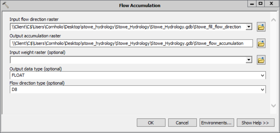
2) Open the Flow Accumulation tool. This tool creates a raster layer that indicates where water is most likely to accumulate. The flow accumulation for each cell is expressed as a numeric value based on the number of cells that flow into that cell. Cells with high values of accumulation often coincide with the locations of flowing water bodies. With your flow accumulation raster, you’ll identify the Little River that flows through Stowe.
- For your Input flow direction raster, choose Stowe_fill_flow_direction.
- Name your Output accumulation raster Stowe_flow_accumulation.
- You’ll leave the remaining parameters unchanged. The first of these parameters applies a weight to each cell, which is useful when you expect water to be distributed in ways that aren’t uniform (for instance, in larger study areas where precipitation levels may vary significantly). The second parameter determines whether accumulation will be measured with integers or floating points. Floating point, the default value, allows for the inclusion of decimal places, making it more accurate in most situations. The third parameter determines the input flow direction.
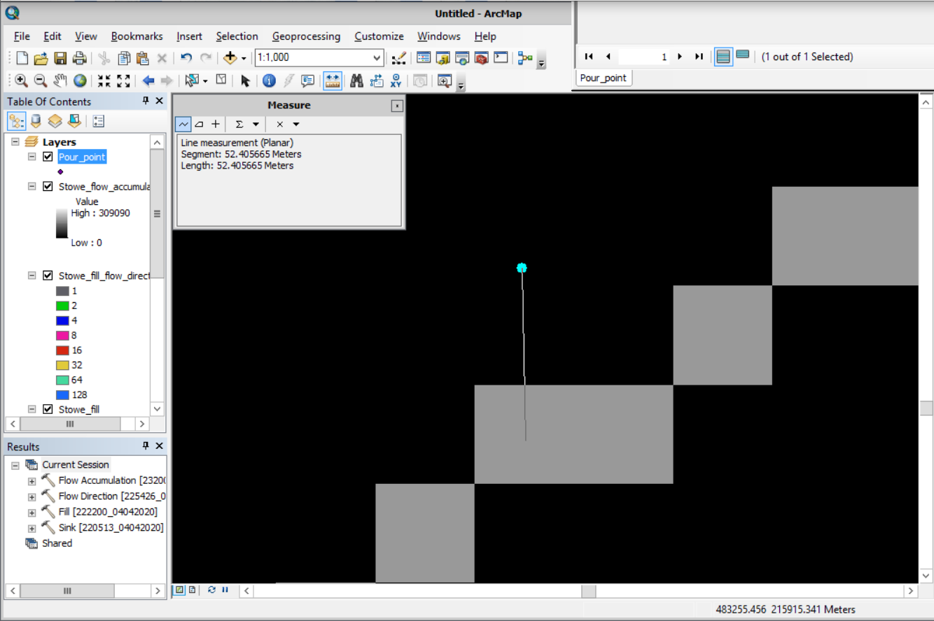
The next step of the task opens the Measure Distance tool (which is a tool on the ribbon, not a geoprocessing tool). You’ll use this tool to measure the distance between the current outlet point and the Little River’s location as represented in the flow accumulation raster. You can use this distance to then snap the outlet point to the correct cell so that it precisely lines up with the stream. Be sure you’re as precise as feasible by zooming in closer to the outlet point. click the outlet point. Then double-click the approximate center of the nearest cell with a high flow accumulation value. The Measure Distance tool’s window updates to include the length of the measurement. I measurement approximately 50 meters so I’ll round to a distance of 60 meters when I snap the outlet point to the stream. A snapping distance that is slightly higher than the measured distance will help avoid ambiguity in the tool. When deciding on a snapping distance, be sure it doesn’t exceed the measured distance by too much, or the point may snap to an area further downstream.
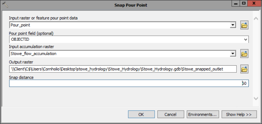
3) Open up the Snap Pour Point tool.
- For Input raster or feature pour point data, choose Pour_point.
- For Input accumulation raster, choose Stowe_flow_accumulation.
- Name the output raster Stowe_snapped_outlet.
- For Snap distance, type 60.
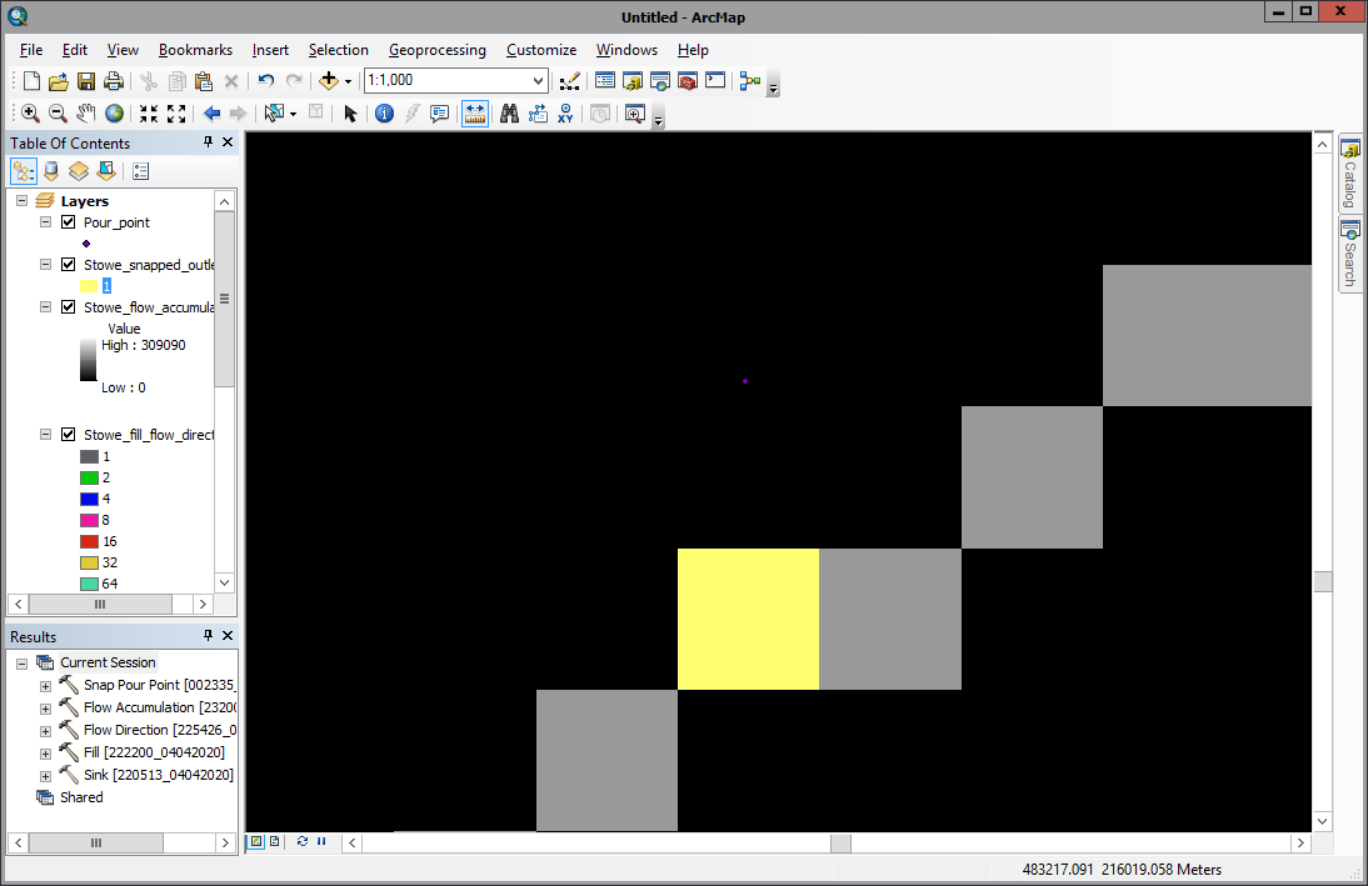
The tool runs and the snapped outlet raster layer is added to the map. The raster displays a single cell that represents the outlet’s new location. In the example image, the snapped outlet is represented as a yellow cell.
Now that you have both a flow direction layer and an accurate outlet layer, you can determine the watershed area upstream of the outlet.
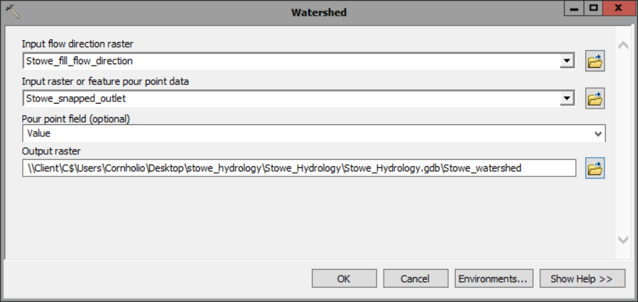
4) The final step of the task opens the Watershed tool.
- For Input D8 flow direction raster, choose Stowe_fill_flow_direction.
- For Input raster or feature pour point data, choose Stowe_snapped_outlet.
- For Output raster, set the name to Stowe_watershed.
Next, you’ll start determining how long it takes water to reach the outlet, allowing the town to better predict when flooding will occur during a hypothetical rainfall event. To determine the time it takes water to flow somewhere, you first need to determine how fast water flows. You’ll calculate the speed of flowing water with a velocity field, another type of raster layer. There are many types of velocity fields, and they can be calculated with a wide variety of mathematical equations. You’ll create a velocity field that is spatially variant, but time and discharge invariant. This means that your velocity field makes the following assumptions:
- Velocity is affected by spatial components such as slope and flow accumulation (spatially variant).
- Velocity at a given location does not change over time (time invariant).
- Velocity at a given location does not depend on the location’s rate of water flow (discharge invariant).
In reality, velocity could be time variant and would definitely be discharge variant. However, incorporating these variants would require additional datasets that might not be available and use modeling techniques that might not be replicable in a GIS environment. The spatially variant, time- and discharge-invariant velocity field will provide a generally accurate result, although it’s important to remember that any method will be only an approximation of observed phenomena. You’ll use a method for creating velocity fields first proposed by Maidment et al. (1996)1. In this method, each cell in the velocity field is assigned a velocity based on the local slope and the upstream contributing area (the number of cells that flow into that cell, or flow accumulation). They use the following equation:
V = Vm * (sbAc) / (sbAcm)
Where:
- V is the velocity of a single cell with a local slope of s and an upstream contributing area of A.
- Coefficients b and c can be determined by calibration. In this scenario, you’ll use the method’s recommended value of b = c = 0.5.
- Vm is the average velocity of all cells in the watershed. You’ll assume an average velocity of Vm = 0.1 m/s.
- sbAcm is the average slope-area term throughout the watershed. To avoid results that are unrealistically fast or slow, you’ll set limits for minimum and maximum velocities. The lower limit will be 0.02 meters per second, while the upper limit will be 2 meters per second.
This equation is only one of many ways that a velocity field can be calculated, and it comes with several assumptions and limitations of its own.
The primary variables in the equation you’ll use for your velocity field are slope and upstream contributing area. You already have a raster layer for upstream contributing area: the flow accumulation layer you created above, but we don’t yet have a slope layer, so that’s the next one we’ll create.
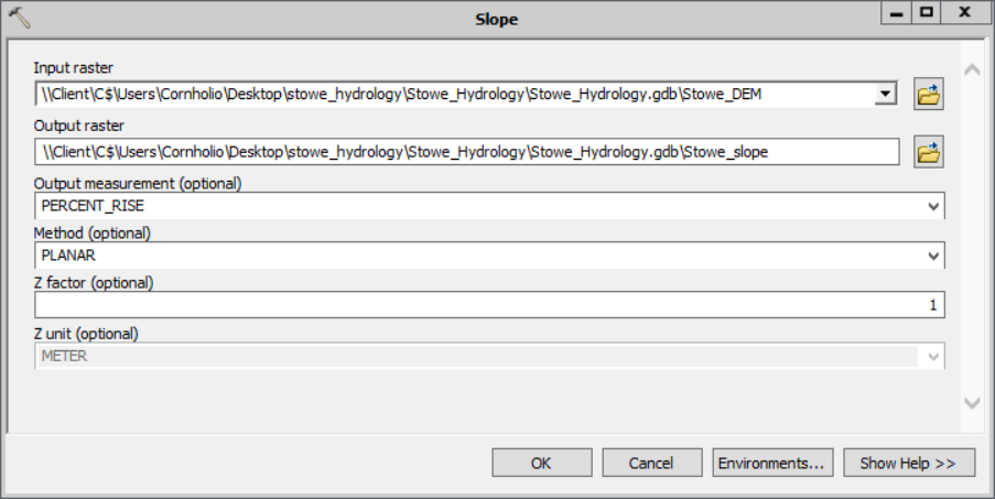
1) Open the Slope tool.
- For the Input raster, choose Stowe_DEM
- Name your Output raster Stowe_slope
Now that we have a raster layer for both slope and flow accumulation area, we’ll calculate a new raster layer that combines them. This layer will show the slope-area term (the value sbAcm from the Maidment et al. equation).
2) The next step can be accomplished using the Raster Calculator tool.
- Use the fields to create the expression:
Power("Stowe_flow_accumulation",0.5) * Power("Stowe_slope",0.5) - Name your output raster Stowe_slope_area_term.
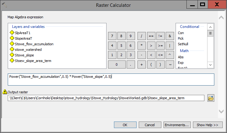
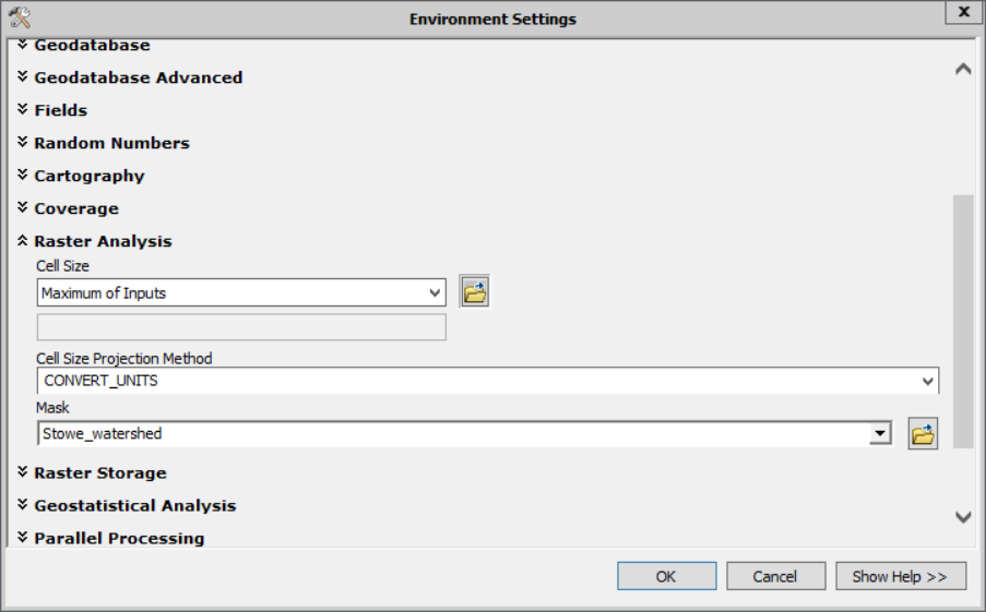
- Finally, lets use the environments of this tool to clip to our watershed at the same time: In the tool parameters, click Environments. Under Raster Analysis for Mask, choose Stowe_watershed.
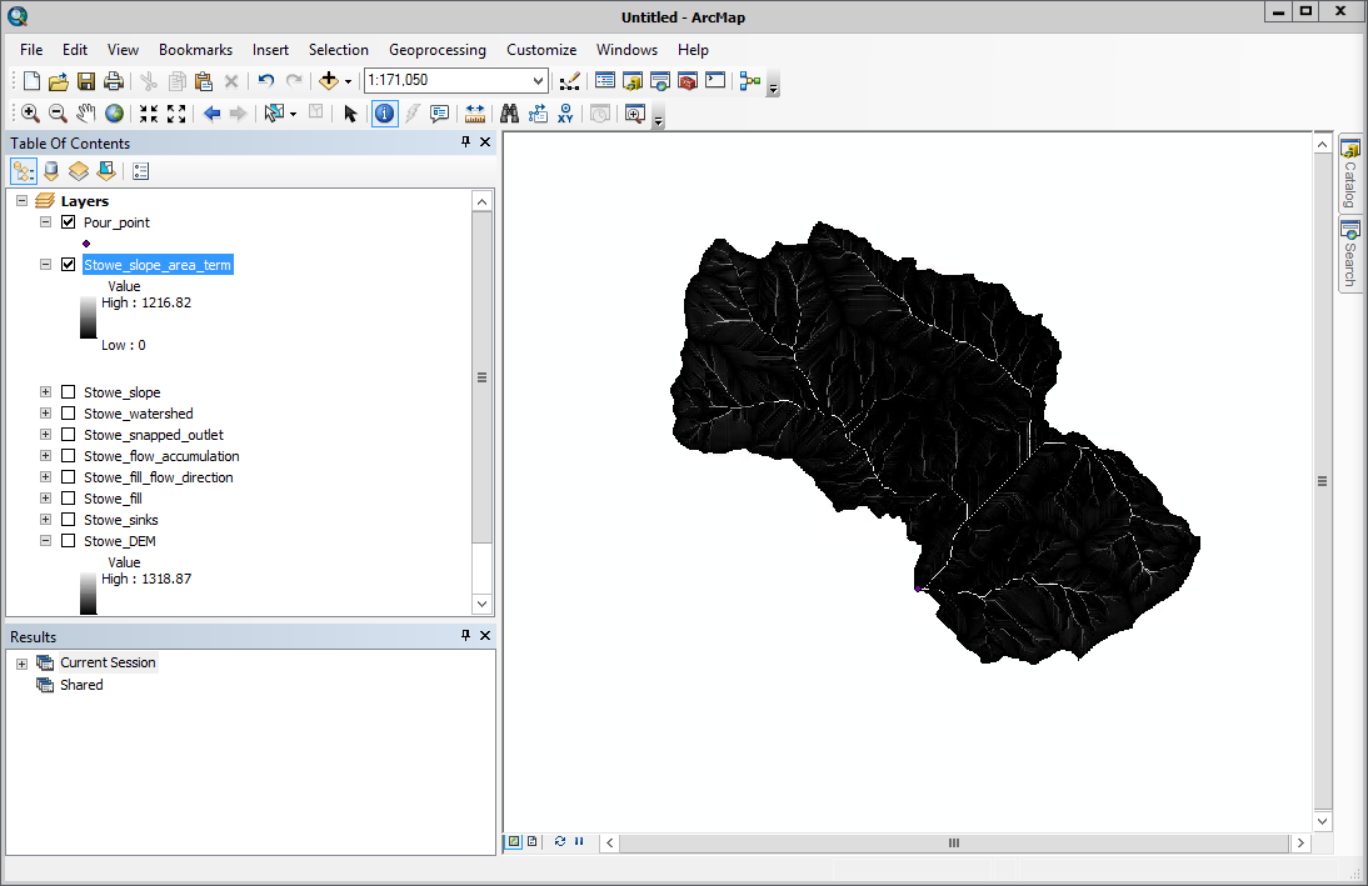
Your output should look like so:
3) Now that you have the slope-area term, you can calculate a velocity field using the following equation:
V = Vm * (sbAc) / (sbAcm)
As mentioned previously,
- Vm is the average velocity of all cells in the watershed. You’ll use an assumed average value of Vm = 0.1, which is recommended by Maidment et al.
- Similarly, sbAcm is the average slope-area term across the watershed. Because you’ve calculated slope-area term for the watershed, we can simply pull the median out of our raster. To find it you need to…
3A) right-click Stowe_slope_area_term and choose Properties, and under the Source tab and expand the Statistics heading.
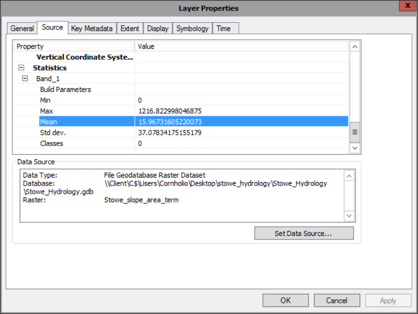
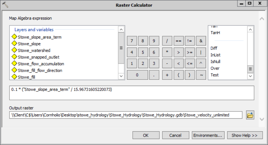
3B) and then open a raster calculator and enter the expression, Where [Mean slope-area term] is the value that you copied from the Layer Properties window:
- You expression should look like:
0.1 * ("Stowe_slope_area_term" / [Mean slope-area term]) - Call that output Stowe_velocity_unlimited
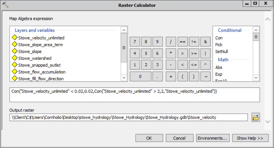
The raster layer you created is a velocity field, but it has unrealistically high and low velocities. For instance, some values in the field have a velocity of 0 meters per second, which is unlikely during an extreme rainfall event. Likewise, the maximum value of approximately 7.5 meters per second is unrealistic even during a major flood. You’ll limit the velocity values with a lower limit of 0.02 meters per second and an upper limit of 2 meters per second. Bearing in mind that there are a number of ways to end up with the desired output, the most direct in my opinion is a complex raster calculator con expression. Other alternatives include reclassifying, multiple con tools, or a clamp tool to name a few.
4) Open up a Raster Calculator and enter your expression.
- My expression looks like so:
Con("Stowe_velocity_unlimited" < 0.02,0.02,Con("Stowe_velocity_unlimited" > 2,2,"Stowe_velocity_unlimited"))- Read it from right to left: “If “Raster” is less than x, put y, otherwise; if “Raster” is greater than than w, put z, otherwise put “Raster””
- Save your output as Stowe_velocity.
Having now created a velocity field that predicts how fast water will flow throughout Stowe, we still need to know the time it takes to get to the pour point. In this step we’ll create an isochrone map, which maps the time it takes to reach a specified location from anywhere else in an area. To create the isochrone map, you’ll first create a weight grid. Then, you’ll assess the time it takes for water to reach the outlet.
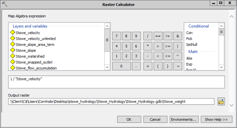
Flow time is calculated with a relatively simple equation: The length that water must flow divided by the speed at which it flows. While you know how fast water flows due to your velocity field, you don’t know flow length. To determine flow length, you need two variables: flow direction (which you know) and weight (which you don’t). Weight, in regard to flow, represents impedance. For instance, water flowing through forested land takes longer than water flowing over smooth rock because it’s impeded by terrain. While calculating weight may seem difficult without detailed terrain data, we can simplify our model by assuming that this weight is the inverse of the velocity we calculated. This is more formally notated as
Weight [L-1T] = 1 / Velocity [LT-1]
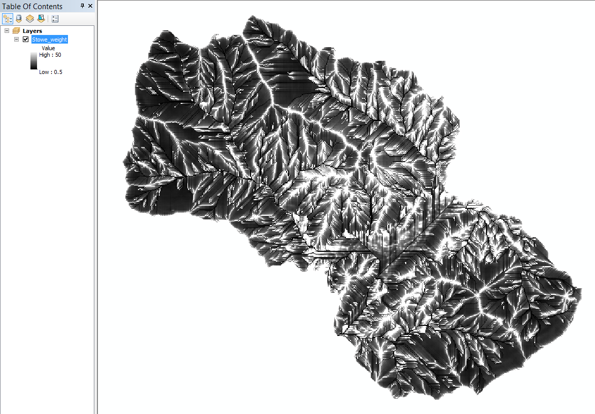
1) Thus, it is a simple matter to create our weights grid with a raster calculator.
- The raster calculator expression is:
1 / "Stowe_velocity" - Save the output as Stowe_weight
- Your output should look like so:
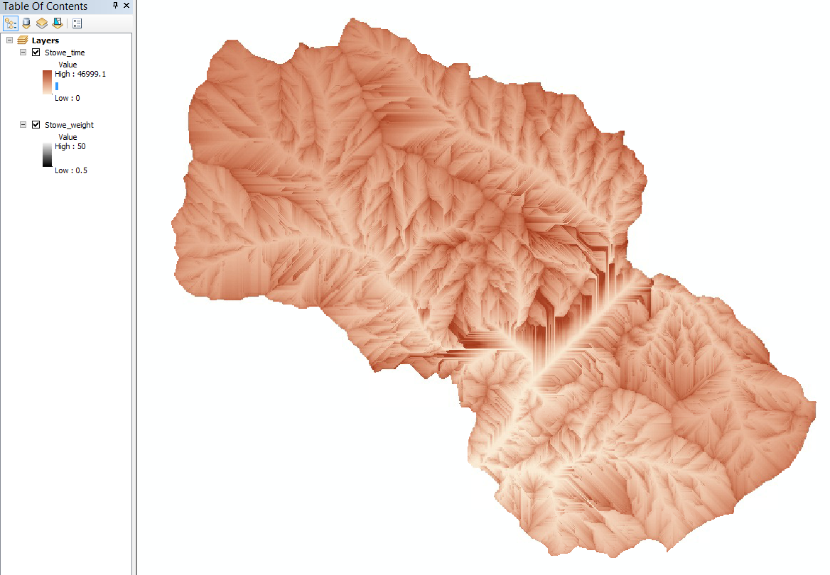
2) The next step of the task uses the Flow Length tool. While this tool, as its name suggests, normally calculates flow length, it has an optional parameter to include a weight raster. When a weight raster is included, the tool calculates flow time instead.
- For Input flow direction raster, choose Stowe_fill_flow_direction.
- For Output raster, name it Stowe_time.
- For Direction of measurement, confirm that Downstream is chosen.
- For Input weight raster, choose Stowe_weight.
- Finally, use the environments of the tool to clip to our watershed at the same time again.
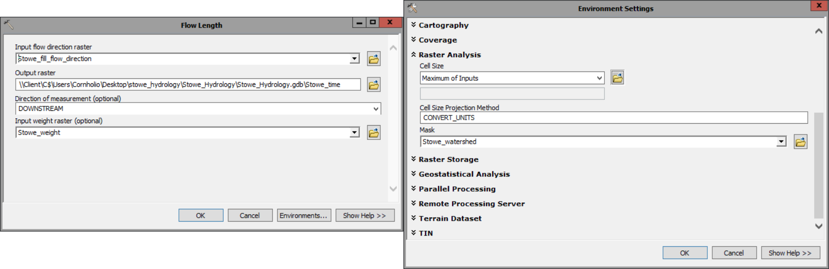
- Your output should look like so, and has units of seconds.
The last step we want to accomplish is to create a unit hydrograph. In essence, this unit hydrograph is the area that falls within the specific we want the histogram of the output layer. Although conceptually simple, this can be quite difficult, as outlined in the source tutorial. Fortunately, simpler solutions exists, and the exact method will vary depending on your desired output. Here I will show how to create a “raw” unit hydrograph and manipulate it within Arcmap and Microsoft Excel.
Approach 1) Visualize a “raw” unit hydrograph histogram and then Extract to create the desired output
We will first…
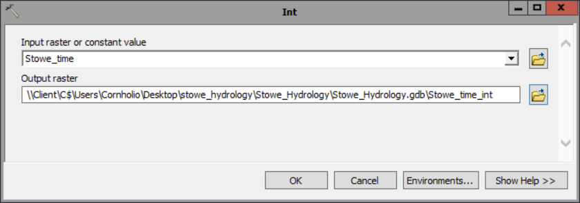
1) Cast the raster to an int. Because our unit is seconds, truncating our numbers is a reasonable tradeoff, and has the added benefit of creating a workable attribute table for us to export.
- The input raster is Stowe_time
- Save the output as Stowe_time_int
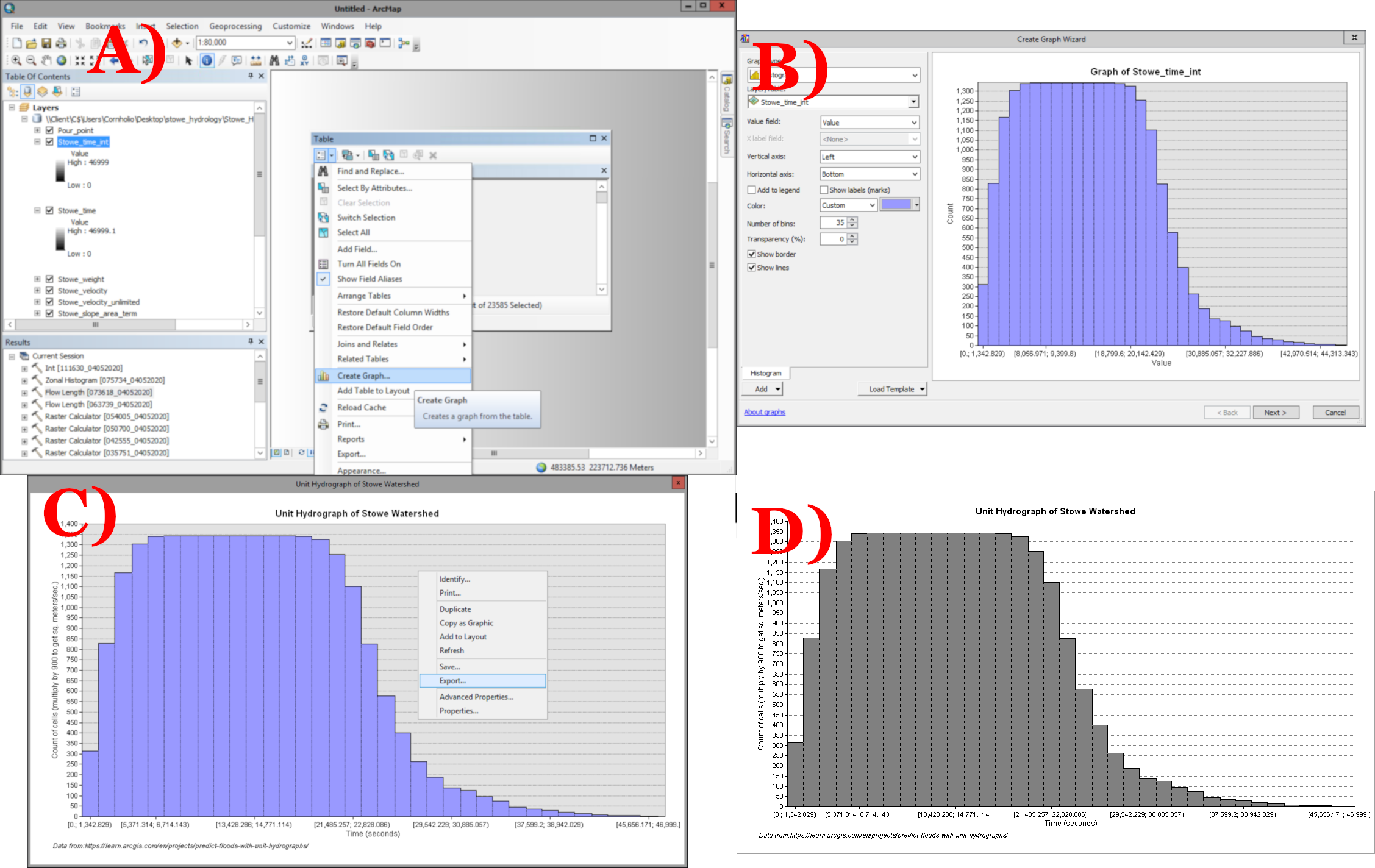
2) Export our results. We can export the raster as a table and use another software package to make a graph, or we can use ArcMap’s built in graph maker to create a simple graph.
2A) Open the attribute table and create a graph,
2B) Set the axis value to value and the number of bins to something sane (I started with 35). Click next and click finish.
2C) Right click on the graph and change advanced properties, or export the image
2D) A final graph.
3) Lets now export this database and manipulate it within Excel to create a unit hydrohraph. Here I’ll walk you through how to take the exported database into Excel and then transform it into a PivotTable for formatting and visualization.
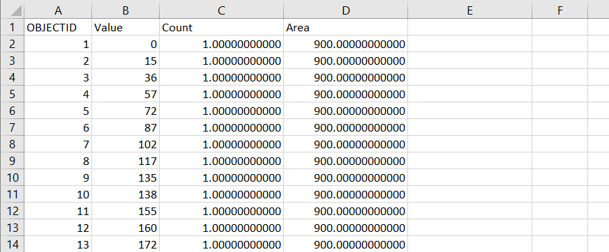
- To export the database, click on the table options and export it to a dbase table on your hard drive (not in a geodatabase)
- From there you can open the table in Excel using File > Open.
- We need to first create a column for area, click in cell D2 and enter the formula
=C2*30*30 - Click the little black box at the lower right hand corner of the cell to fill the formula down.
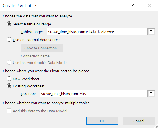
- Go to Inset > pivot table and choose the whole table. Dump the pivot table out in the same worksheet.
- Add Value and Sum of Area to Rows and Values respectively.
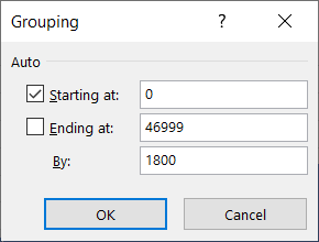
- Click in the first column of Value in the pivot table, and click Group Field up in the PivotTable Analyze ribbon
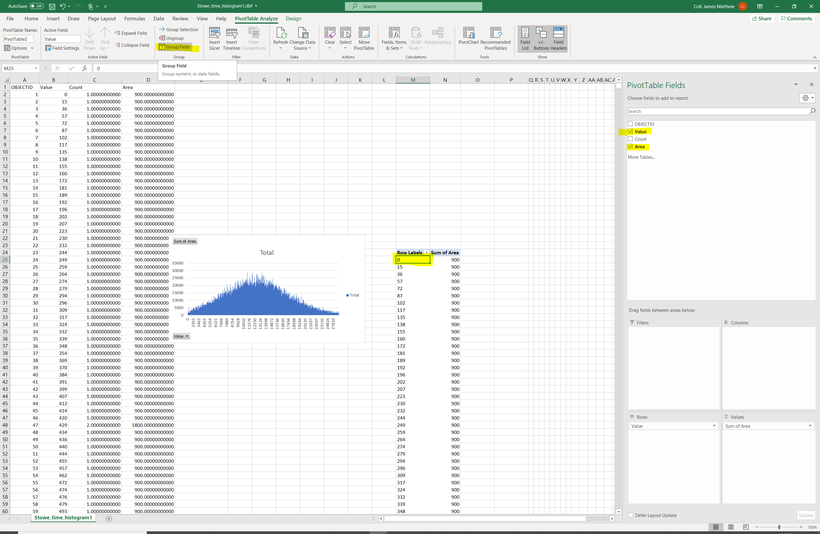
- Group the field into chunks of 1800…
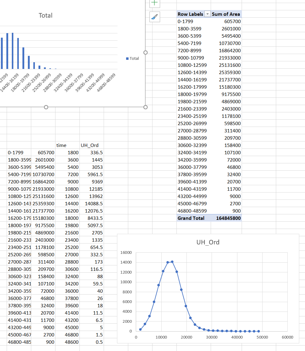
- Copy the table, and calculate the unit hydrograph using a time field and the area divided by the timestep.
1) We can Reclassify our time raster into N isochrones (contours of time) and generate a graph from that. Here I’ll demonstrate a 30 minute timestep (1800 seconds).
- Click the classify button after adding the Stowe_time raster to the input, and set the interval size to 1800 (30 minutes in seconds)
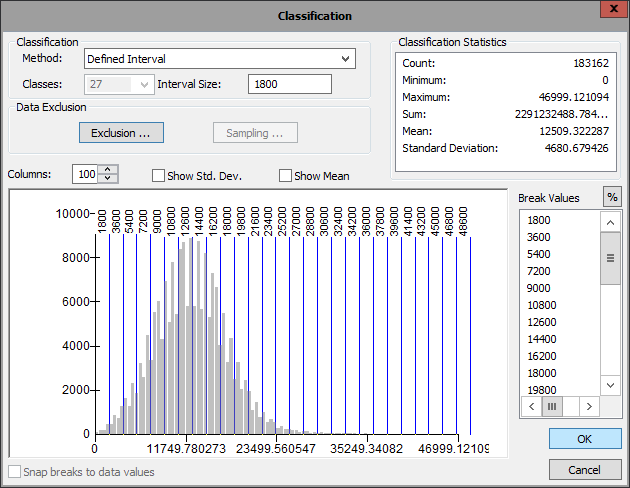
- Name the output Stowe_1800_isochrone.
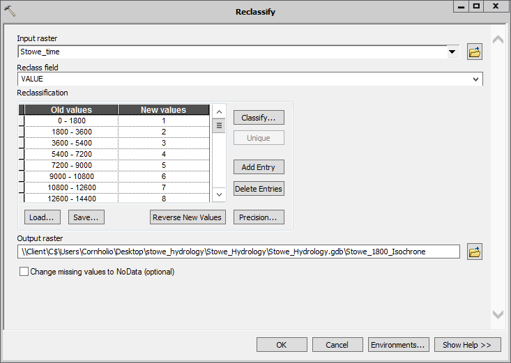
2) Now we’ll use these as the zones to calculate the ordinate of the unit hydrograph. These “ordinates” are the sum of the area within that time step divided by the timestep. In essence, this is the area within the isochrone divided by range of the isochrone. We will first add a new field to the Stowe_1800_isochrone and calculate the area within each isochrone. We will then normalize that area to the time range of our isochrone.
- Use the Add field button in the table options of the Stowe_1800_isochrone raster
- Name the field time and set the type to double.
- Right click on the newly created field and calculate the area (simply the [Value] * 1800)
- Create a new field called area of type double.
- Right click on the newly created field and calculate the area (simply the [Count] * 30 * 30)
- To finish, create a last field called UH_Ord of type float
- Your expression here is the area divided by the range of the isochrone ([Area]/1800)
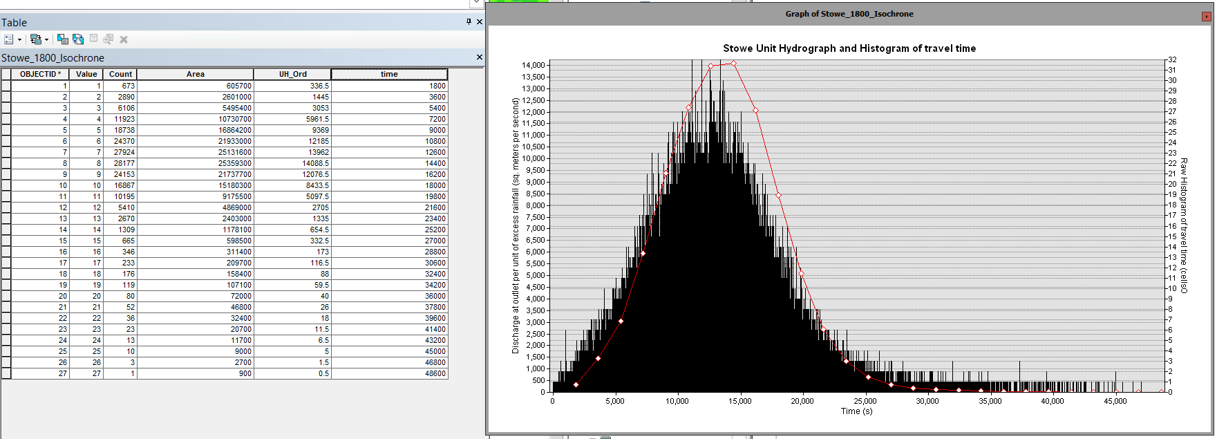
3) Finally, create the graph.
- Explore the graphing options as before. Here I demonstrate how you may add two series to the same graph (here the raw histogram and the aggregated and normalized unit hydrograph.
Answer questions 3 and 4 related to this part of the lab. Submit your final answer sheet to blackboard.
-
MAIDMENT, D.R., OLIVERA, F., CALVER, A., EATHERALL, A. and FRACZEK, W. (1996), UNIT HYDROGRAPH DERIVED FROM A SPATIALLY DISTRIBUTED VELOCITY FIELD. Hydrol. Process., 10: 831-844. doi:10.1002/(SICI)1099-1085(199606)10:6<831::AID-HYP374>3.0.CO;2-N ↩︎