Lab 02 - Cartographic Modeling
This lab will introduce local operations using cartographic modeling (map algebra). Part 1 is intended to show you how you can organize and display raster datasets in a usable format. Part 2 will walk you through how to calculate NDWI and perform a water area analysis. Part 3 you will model the geographic distribution of Kudzu in the conterminous United States and then compare your model to the actual geographic distribution, using Map Algebra and attribute table manipulation. I’ve prefaced each lab with the learning objectives of the exercise, what you need to submit to blackboard, a set of materials for the lab as appropriate, and then the instructions for the lab.
Outline:
Hint: Copy and paste the questions below into a word document and submit it to blackboard
*** # **Materials** [click to download](https://kansas-my.sharepoint.com/:f:/g/personal/j610c377_home_ku_edu/EuPaly9t2yxGrCruD_fcGakBSzTfsGwq5KC-iWYwU6GNog?e=YznxCc)
| Relevant part | Data Name | Description |
|---|---|---|
| Part 1 | BaseData | Data we downloaded as part of lab 1 |
| Part 3 | usanpre25k | annual precipitation in mm (25000m grid) |
| Part 3 | usfrost25k | number of frost-free-days in conterminous US (25000m grid) |
| Part 3 | sample1.shp | point file showing locations of known presence/absence of Kudzu (to be used to make model) |
| Part 3 | sample2.shp | point file showing locations of known presence/absence of Kudzu (to be used for accuracy assessment) |
If you are short on space, you only need the .mpk from part 2, the LANDSAT tiles are ~20 gigs and are provided for reproducibility’s sake.
- Open up a new ArcMap document.
- First, a few housekeeping items. Let’s take the training wheels off ArcMap and make sure we can overwrite data. Click Geoprocessing > Geoprocessing Options and make sure the top two boxes in this window are selected. You may also want to increase the time period results are stored to a month or so.
- From the 1995 year, add in the green, NIR, MIR, and MTL bands/images.
Hint#1: When performing the NDWI calculation, we refer to bands based their wavelength (e.g. green, NIR). However, when distributing data the bands are referred to by their number based on sensor properties (so in our case, LANDSAT 5 TM has 7 bands and change). GEE provides a nice, concise overview of a remote sensing products bands, see https://developers.google.com/earth-engine/datasets/catalog/LANDSAT_LT05_C01_T1
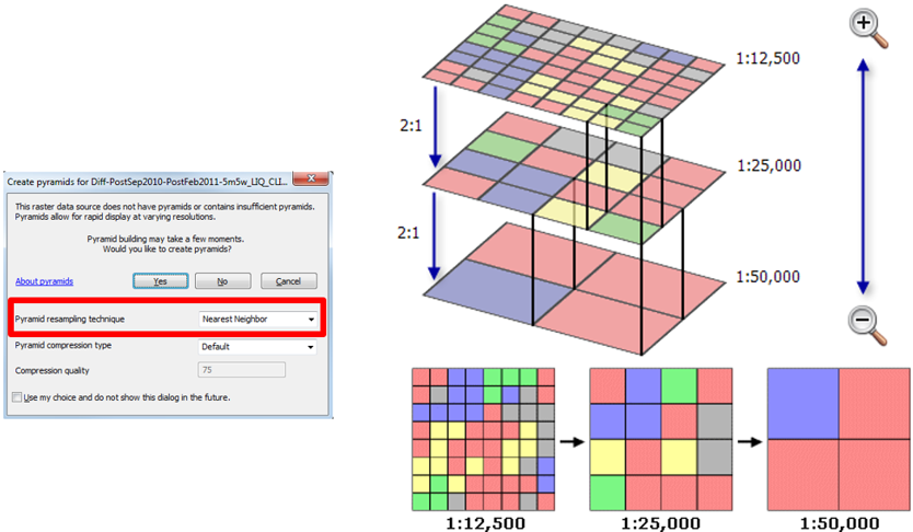
A note about pyramids: You will want to build pyramids when you add raster images into ArcMap. You will notice that when this is done, ArcMap will create a file with a .ovr extension (look using the Windows file browser). We’ll talk about pyramids in class more, but as a cursory introduction, think about Google Maps. When you zoom out to look at the entire planet, there is no physical way to represent 30 meters on the screen. Instead, we take a generalization of all the pixels underneath the region and display those values in their place. Because Google sets the standards for mapping, there are generally 21 levels of images that are loaded in, with the top most layer being zoom level 1, and increasing as you zoom in. See an interactive example of this concept in action at https://www.maptiler.com/google-maps-coordinates-tile-bounds-projection/
- Select all 4 images using shift-click, and right click > Group to place them in a group. Slow click and rename this group to LS1995

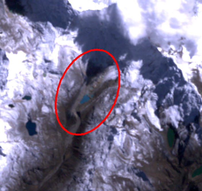
- Finally, let’s find our lake using the go to xy tool and copy/pasting the lat/long in: -9.3970552,-77.3802742
Note: Skill review from Lab 4
- We next need to create a shape representing the area of analysis. First, right click on your BaseData folder and create a new File Geodatabase. Rename the database to LakePalcacocha.gdb
- Right click on the new geodatabase and go to New > Feature Class
- Name the Feature Class AOI and set the type to polygon. Click next.
- Scroll to the bottom of the window, expand the Layers folder, and click on the only option (WGS_1984_UTM_Zone_18N | WKID: 32618). Click through the rest of the setup dialog to finish creating the shapefile. Assuming you were successful you should now have a new layer called AOI in your TOC
- Start an editing session (Editor toolbar > Editor > Start editing)
- Make sure you are editing the AOI layer/LakePalcacocha.gdb database.
- On the editor toolbar, click create features
- Click on AOI to bring up the construction tools
- Use the Circle tool to create a small circle that encompasses the entirety of the lake. It is alright for our purposes if we include land area, but do not make it so large that it might include nearby lakes. This should look something like so:
- Click on the editor and stop editing. Save your edits when it prompts you to.
- The NWDI is defined as the normalized difference of the Green and Near Infrared bands of the Thematic Mapper. (See the McFeeters paper in the International Journal Of Remote Sensing)
$$NDWI = \frac{Green-NIR}{Green+NIR}$$ - We will use the raster calculator tool to accomplish this. At this point we can also use the environmental settings to clip our data so we don’t process the whole scene.
- Go to Geoprocessing > Environments
- Under workspace, point the Current and Scratch workspaces to our LakePalcacocha.gdb
- Under processing extent, set the extent to “Same as Layer AOI”. Click OK
- Use the search bar to pull up the Raster Calculator and use the prompts to calculate the NDWI.
Extension warnings? Did you take the time to read it? Warnings are a chance for programmers to communicate to you and in this case you should learn that you need to turn on spatial analysis under Customize > Extensions.
- Go ahead and try to enter in the expression above. Save the resulting raster using the folder icon under the Output Raster dialog box, click on the name of one of the other bands (to preserve the LANDSAT naming convention), and change the end of the file to …NDWI.tif.
You’ll notice that the resulting raster has a value of 0, and is entirely empty. This is because ArcMap likes to save memory and forces raster calculations to integers. Fixing this just means we need to be more verbose and run the calculations as floats using Float() under the Math section. This conversion to integer occurs in both the numerator and denominator, so the float needs to wrap both of them separately.
- Go to Geoprocessing > Results.
- If you double click on the last tool run, it will open the tool prompt as it was run.
- Change the expression to:
Float(“LT05…B 2.TIF” - “LT05…B4.TIF”) / Float(“LT05…B2.TIF” + “LT05…B4.TIF”)
- The MNWDI is defined as the normalized difference of the Green and Near Infrared bands of the Thematic Mapper. (See the Xu paper, also in the International Journal Of Remote Sensing) $$MNDWI = \frac{Green-MIR}{Green+MIR}$$
- Because this process is so similar to the NDWI (we use band 5, not band 4), it is easiest to pull the results up from our last raster calculator and change a few characters. Change all 4’s to 5’s and change the output file name to MNDWI.
- go to geoprocessing > Results and double click on the last tool run.
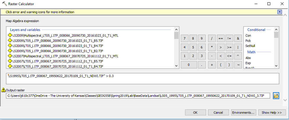
- You’ve probably noticed by now, but the NDWI and MNDWI calculations return an image with valid values from -1 to 1, but this doesn’t tell us what is and is not water. To do that we need to classify the image into a binary water/not water schema. There are a variety of ways to do this that range in sophistication/robustness, but for our purposes, a simple threshold will suffice. This means we want classify all pixels with a NDWI/MNDWI value greater than or less than some value into water.
- Use the identify button and poke around the image to find a good threshold. I settled on 0.30
- Use the raster calculator to select the cells greater than 0.30, and append the name of the NDWI layer with the threshold value (…NDWI_3.tif).
 Examine the outputs (right click on the resulting layer and see the attribute table.) You now have enough information to answer the following questions.
Question 1:
Based on the results from 1995, which water delineation metric would you choose to perform this analysis, NDWI or MNDWI. Why?
Question 2:
What is the area of the lake in 1995?
Question 3:
Calculate the area of the lake for 2003 and 2009. Finish the table below and create a short graph of the area through time. Create a short map of the before/after.
Year # of Pixels 1995: xxx 1997: 100 1999: 143 2001: 184 2003: xxx 2005: 437 2007: 503 2009: xxx 
One of the downfalls that plague many passive remote sensing platforms is the inability to penetrate cloud cover. Notice that although we didn’t happen to encounter cloud obfuscation in the first part of this lab, clouds are not uncommon. Let’s use water year 2005 as an example. I’ve taken the liberty of downloading and setting up your ArcMap document and data for you. Just download the Map package and double click to open.
- Because land/water has a lower reflectance across all bands as opposed to clouds, one of the simplest and most effective means of filtering out cloud cover is to take the local minimum from a raster stack.
- ArcMap has a tool called Cell Statistics which performs statistics for local operations. Either use the search tool or find it in Spatial Analyst Tools > local.
- We want to calculate the minimum of each band within the 4 seasons. Using band 4 for the winter as an example, the inputs should look like so:
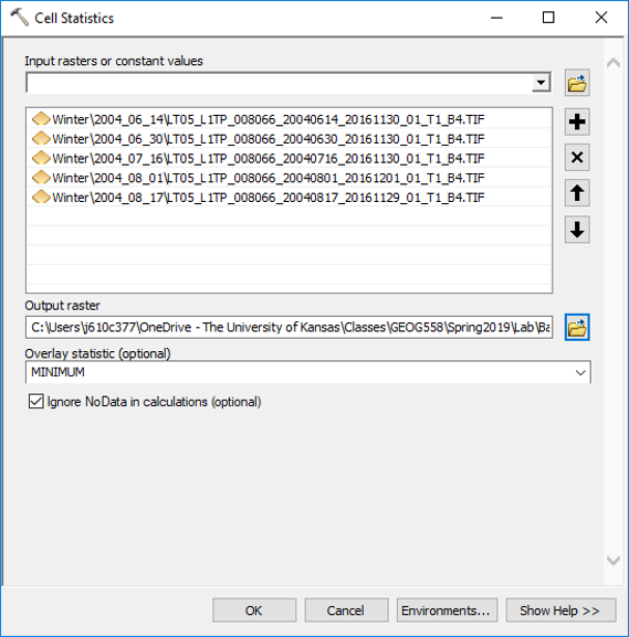
- I have gone ahead and taken the minimum of 3 of the 4 seasons. So you only need to calculate the minimums for the spring months.
- Perform the NDWI calculation, thresholding, and area measurement as was performed above.
- Answer questions 4 and 5 below. Save and close Arcmap, we’re done looking at the lake for now.
Question 4:
Create another graph of lake volume over time as was performed above.
Question 5: What are some potential issues of using gap-filled imagery for scientific analysis?
- Start ArcMap and add sanpre25k, usfrost25k, and sample1 from your lab02\Part03 folder.
- extracting data for building Kudzu distribution model.
- Open the attribute table for sample1.
- The numbers in the “KUDZU” field represent presence or absence of Kudzu at that point (1 for presence, 0 for absence)
- You want to find the minimum annual precipitation (in mm) and the minimum frost-free days at each of these points. This information will be your source of input for modeling potential Kudzu distribution across the U.S.
- Close the attribute table.
- ArcToolbox contains an Extract values to points tool that will add the value of a raster to a set of points. It then creates a new point file with an attribute holding that raster value.
- In the Spatial Analyst Toolbox >Extraction > Extract values to points tool.
- This tool requires three inputs and has two optional ones. You can find out more information about each of the inputs (this applies to other ArcTools as well) by clicking on the Show Help button and then clicking on the field of interest.
- Set your Input point features to sample1 (You can either use the drop-down that shows all the point layers in the ArcMap Table of Contents or the Browse file button to navigate to the file).
- Set your Input raster to usanpre25k.
- Set Output point features so that it saves the new file called sample1precip to your lab02\Part03 folder.
- Click OK (Be patient. This may take a while.).
- Your new point file will appear in the ArcMap Table of Contents.
- Open the attribute table for sample1precip.
- Notice the new variable called RASTERVALU that contains the annual precipitation amount for that point
- Repeat the above steps to create a similar point file containing a RASTERVALU attribute for frost-free days at each point. Call it sample1frost.
Alternatively, there is an Extract multi values to points tool, which will do this whole process at once.
By looking at the minimum precipitation and minimum number of frost-free days that Kudzu required for survival in the sample points, we can model (predict) its potential geographic expansion across the U.S. In order to do this, we need to get this information out of the datasets we just created. To find the minimum annual precipitation and minimum number of frost-free days required for Kudzu to survive:
- Open the attribute tables of your samples and perform an attribute query to select only those points with known Kudzu presence (“KUDZU” = 1)
- Show only the selected records using the table toggle button.
- Sort in ascending order the RASTERVALU field (R-Click on column heading).
Question 6:
The minimum annual precipitation for Kudzu to survive is:________?
Question 7:
The minimum frost free day for Kudzu to survive is:________?
- Create new grids based on the usanpre25k and usfrost25k grid using Raster Calculator
- usanpre25k >= minimum value** (**Minimum Value in question 6)
- From the usanpre25k, the new grid cells with an annual precipitation greater than or equal to the minimum annual precipitation will have a value of 1, while cells with an annual precipitation less than the minimum value will have a value of 0
- Save the grid as precipitation in your lab02\part03 folder
- usfrost25k >= minimum value** (**Minimum Value in question 7)
- From the usfrost25k, the new grid cells with a frost-free-days greater than or equal to the minimum frost-free-days will have a value of 1, while cells with a frost-free-days less than the minimum frost-free-days will have a value of 0
- Save the grid as frost in your lab02\part03 folder
- Predict the Kudzu U.S. distribution by multiplying the precipitation and frost grids. Save the output grid as kudzu_model.
Question 8:
The total area (in m2) suitable for Kudzu to survive (according to your model) is:________ (m2)
- Add sample2 to your ArcMap Table of Contents
- Using the Extract values to points tool you now want to create a new point shapefile called sample2check that will have an attribute of actual presence (KUDZU) and one for predicted presence (RASTERVALU found by using kudzu_model as raster input)
After you have created sample2check you can quantify your accuracy in one of many ways. Here are two suggestions:
- Add a new field named check and perform the following calculation: check = [RASTERVALU] * 10 + [KUDZU]. The Check field should have the following outputs: 0, 1, 10, and 11 (0 and 1 represent 00 and 01 respectively)
- Perform attribute query using the AND operator 4 times, once for each possible combination. (i.g. KUDZU = 1 AND RASTERVALUE = 0)
Question 9:
Complete the following table:
Actual Kudzu Distribution No Kudzu Kudzu Your Model No Kudzu D:(00) B:(10) Kudzu C:(01) A:(11)
Use your constructed confusion matrix and the accuracy metrics below to help answer question 10. For more about confusion matrices look at wikipedia:
Accuracy - ((A+D)/(A+B+C+D)):
False Positive Rate - (C/(A+C)):
False Omission Rate - (B/(A+B)):
MCC - (A*D-B*C)/sqrt((A+B)*(A+C)*(D+B)*(D+C)):
Question 10:
Discuss some of the reasons for the inaccuracy of your model. In particular, examine why the error may be occurring. Also, looking at your kudzu_model layer, where geographically do you think this error is? (Hint: Consider the factors that your model did not include that could explain the geography of the model’s error)
Need help answering question 10? Make a map like so! Useful tools: Raster to polygon, symbology as categories, rectangle as text, insert images. If performance is an issue, add basemaps last. Spend some time on the map and I’ll count that as a response to the question, so throw on a nice album (one of my current favorites) and cartography away!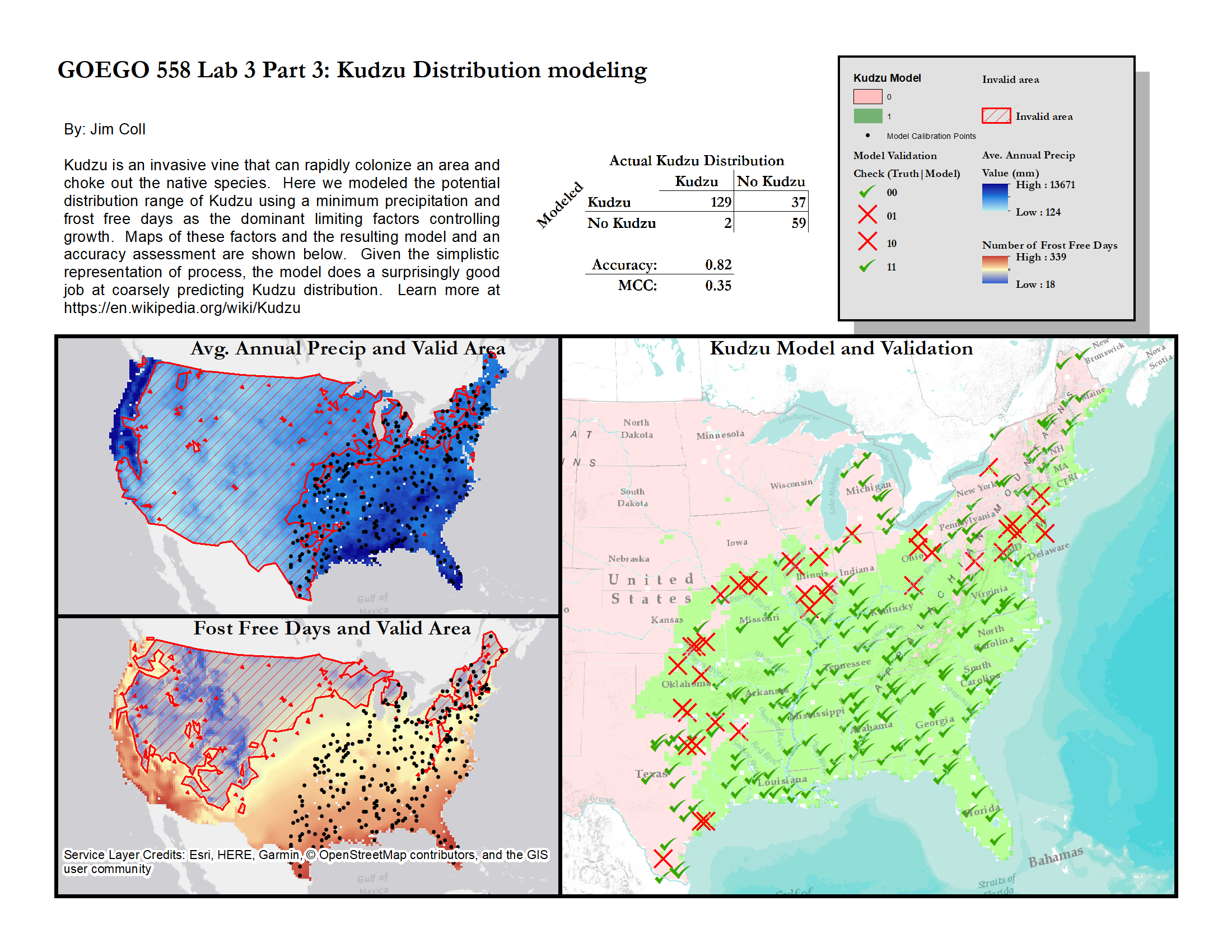
Feel free to save your map document