GEE

Google Earth Engine (GEE) is a cloud-based data and analysis platform which combines more than 17 petabytes of geospatial data, analytic APIs, and a web based Integrated Development Environment in one package and runs on Google’s computational infrastructure, enabling interactive earth data analyses on scales not previously feasible. This platform was first introduced to the public in 2013 as a means of performing an analysis of global forest cover change, published in Science (Hansen et al., 2013). In this flagship application, the authors sought to quantify the spatial distribution and global state of forest loss and gain from 2000 to 2012 by blending more than 654,000 Landsat scenes across the 12 years of the analysis — the resultant analysis of 700 Terapixels of data took more than 1 million hours of computation and exported results in a comparatively trivial 4 days across the Google compute infrastructure.

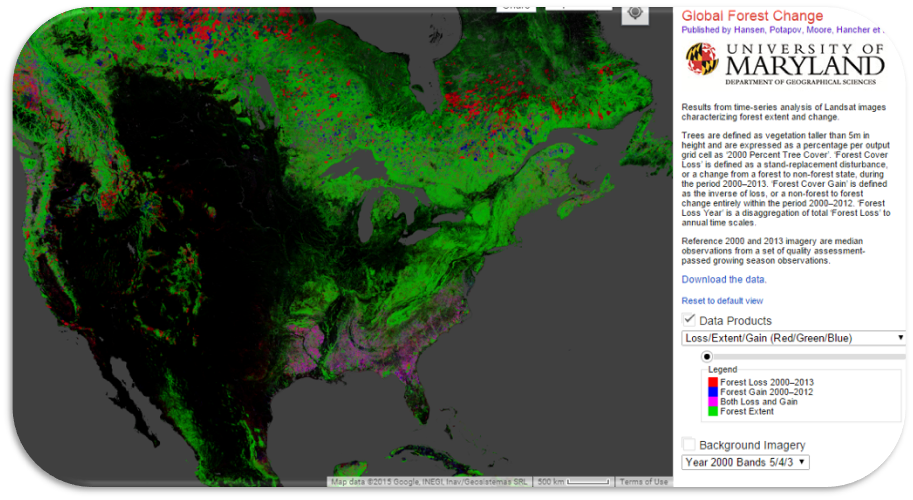
Such analyses once used to sit behind such extreme barriers of entry that no one would have been able to produce, much less reproduce, these results.

To use GEE, you will need to request a user account at https://signup.earthengine.google.com/#!/. Once approved, you have access to the datasets and the Google computation infrastructure. This access takes the form of a REST API. There are currently two means of doing so, one Python based, and the other JavaScript based. The less popular of the two methods, the Python library, allows users to interact with Earth Engine using the Python programming language. The Google Earth Engine API guide has a full walk through of how to install the needed libraries, and is available at https://developers.google.com/earth-engine/python_install. The more popular means of accessing GEE is through the JavaScript library which is accessed through a web-based IDE, more commonly called the Code Editor, by pointing a browser at https://code.earthengine.google.com/ and logging in with an authorized GEE account. Although not specifically required, it is recommended that you use Google Chrome, and as this is the most popular means of accessing GEE the rest of this entry will be written using the JavaScript IDE. Don’t worry if you are more familiar with Python, the transition to JavaScript is relatively painless and primers are available at https://developer.mozilla.org/en-US/docs/Web/JavaScript/Guide/Introduction. One of the first steps for those new to GEE is to explore the features of the JavaScript API. In the upper right-hand corner of the code editor, click on help > Feature Tour to take a quick guided tour of the platform.

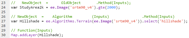
Broadly speaking there are 3 major types of operations one can perform in GEE: Methods, Algorithms, and Functions. The general structure of these are exemplified in Figure 1. Methods require an object to act on and take inputs, as exemplified in Figure 1, line 24, where we query the SRTM dataset for all values greater than 2000. Algorithms are objects themselves and take a specific input to return an object, as exemplified in Figure 1, line 27 where we use the Terrain algorithm to create a hillshade image from SRTM. Functions take an input and do something within the API, as exemplified in Figure 1, line 30, where we add the Hillshade layer to the map.

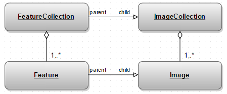
Data objects in GEE are slightly different from more traditional desktop GIS software, but the concepts are very similar. These differences are most pronounced with the data structures outlined below in Figure 2. What GEE calls Images can be thought of as Rasters, and just as Rasters may have more than one band, so too may Images. What GEE refers to as an ImageCollection are simply a collection of Images. What GEE refers to as Features are analogous to features in a shapefile or geodatabase, so FeatureCollections are analogous to the larger shapefile or feature classes in a geodatabase. These data structures also borrow concepts from Object Oriented Programming (OOP) in that Feature can be thought of as the parent of Image and likewise ImageCollections are children of FeatureCollections. Therefore, many of the methods and operations available for Features and FeatureCollections are inherited by Images and ImageCollections.

GEE hosts more than 17 petabytes of publicly available data which can be redistributed. However, users also have the option to upload their own data in popular GeoTIFF or shapefile formats for ingestion into the system as user assets. Assets are limited to 10 GB in size, and are counted as part of your shared Google storage quota (spread across Gmail, Google Drive, ect.). Once in the platform, they are treated the same as any other dataset in the platform and can be shared with other users.

GEE handles many of the concerns typically associated with data preparation, such as storage, cataloging, and projecting the data appropriately. GEE has ingested many of the most popular remote sensing data from various satellite platforms such as LANDSAT, MODIS, and Sentinel to name just a few. The full collection can be browsed at https://developers.google.com/earth-engine/datasets/catalog/. When ingested, the data is stored in its native projection and format to preserve data integrity, and the metadata necessary to effectively use them is also included in each image as properties. Users may inspect, project, and resample the data as necessary, but because the GEE team takes care of these details when the data is ingested, the “time to science” is rapidly accelerated and users are free to spend that time on the analysis and presentation instead of the relatively canned portion of data preprocessing. By using the Search Box at the top of the IDE, you can find relevant datasets and explore how they can be used in GEE.

When working with data in GEE, there are two types of operations we can perform over the data, mapping and reducing. Mapping applies a function to each image in a collection, so a stack of n elements results in a transformed stack of n elements, and is useful when we need to do something to every image (for instance, calculating NDVI over a timeseries of images). Reducers on the other hand take one or more input features and return a reducer number of outputs. These often take the form of conventional map algebra expressions. These expressions can be as conceptually simple as pulling the maximum value of a stack of pixels in an ImageCollection to as complex as non-parametric trends of slope or regional reducers.

Joining data is a hallmark of geospatial analysis, and GEE provides several ways in which different datasets may be joined together based on a specified condition. These conditions, or filters as they are called in GEE, can be spatial, tabular or temporal in nature. GEE applies the conditional filter, and items in the input collections that match the conditions are saved in the output collection depending what output the join wants to keep.

GEE has several image classification methods built into the API. These include unsupervised and supervised classifiers. As of the time of this writing, these include: Cart, Naïve Bayes and Continuous Naïve Bayes, Decision Tree, Gmo Linear Regression and Max Ent, Ikpamir, Minimum Distance, Pegasos linear, and Polynomial, and Gaussian, Perceptron, Random Forest, Spectral Region, Scm, and Winnow. Additionally, if provided with training data, a confusion matrix can be calculated from that classification to present an accuracy assessment.

Although it is often more efficient to perform your desired analysis within GEE, exporting your results for further specialized analysis or publication can come in several forms depending on the desired purposes. This might include CSV files of time series, images, web map tiles, and videos. In addition, a suite of standard JavaScript User Interface (UI) items are available within the IDE which enables users to rapidly design and prototype user interfaces to include items such as combo and check boxes, sliders, and legend elements. These powerful features allow users to publish advanced and fully fleshed out web applications so that those who don’t have a GEE account can interact with or export analysis without looking at a single line of code.

Let’s use GEE to perform one of the most common

// Get an image using its ID
var image = ee.Image('LANDSAT/LT5_L1T/LT50260332010180EDC00'); //an image covering KC
print(image)

// Examine image properties/metadata
// Get information about the bands as a list.
var bandNames = image.bandNames();
print('Band names: ', bandNames); // ee.List of band names

// Get projection information from band 1.
var b1proj = image.select('B1').projection();
print('Band 1 projection: ', b1proj); // ee.Projection object

// Get scale (in meters) information from band 1.
var b1scale = image.select('B1').projection().nominalScale();
print('Band 1 scale: ', b1scale); // ee.Number

// Note that different bands can have different projections and scale.
var b8scale = image.select('B6').projection().nominalScale();
print('Band 6 scale: ', b8scale); // ee.Number

// Get a list of all metadata properties.
var properties = image.propertyNames();
print('Metadata properties: ', properties); // ee.List of metadata properties

// Get a specific metadata property.
var cloudiness = image.get('CLOUD_COVER');
print('CLOUD_COVER: ', cloudiness); // ee.Number

// Get the timestamp and convert it to a date.
var date = ee.Date(image.get('system:time_start'));
print('Timestamp: ', date); // ee.Date

// Display the image
//set map center and zoom level
Map.setCenter(-95,39,8);
//add the image to the map
Map.addLayer(image,{'bands':['B3','B2','B1']},'Kansas City in natural color');
Map.addLayer(image,{'bands':['B4','B3','B2']},'Kansas City in false color composite');

//import or use Landsat image collection  
//

var  lt5= ee.ImageCollection("LANDSAT/LT5_L1T");
//print('Landsat 5 collection', lt5);


//
//Metadata about the collection
//
// Get the number of images.
var count = lt5.size();
print('Count: ', count);

// Get the date range of images in the collection.
var dates = ee.List(lt5.get('date_range'));
var dateRange = ee.DateRange(dates.get(0), dates.get(1));
print('Date range: ', dateRange);

// Get statistics for a property of the images in the collection.
var sunStats = lt5.aggregate_stats('CLOUD COVER');
print('CLOUD COVER statistics: ', sunStats);

//filter images by time, location, and properties
//

// Load Landsat 5 data, filter by date and bounds.
var ic1990s = lt5
  .filterDate('1990-01-01', '1990-12-31')
  .filterBounds(p69_135)
  //.filterMetadata('CLOUD_COVER','less_than',10);
print(ic1990s)

// Get the number of images.
var count = ic1990s.size();
print('Count: ', count);

// Get the date range of images in the collection.
var dates = ee.List(ic1990s.get('date_range'));
var dateRange = ee.DateRange(dates.get(0), dates.get(1));
print('Date range: ', dateRange);

// Get statistics for a property of the images in the collection.
var sunStats = ic1990s.aggregate_stats('CLOUD_COVER');
print('CLOUD COVER statistics: ', sunStats);

ic1990s=ic1990s.filterMetadata('CLOUD_COVER','less_than',10);
print(ic1990s);

//Access individual images in the collection
//
var i1990 = ee.Image(ic1990s.first());

// Convert the collection to a list and get the number of images.
var secondImage = ic1990s.toList(5).get(1);
//print(ic1990s.toList(5));
print('Second image: ', secondImage);

// Sort by a cloud cover property, get the least cloudy image.
var leastCloud = ee.Image(ic1990s.sort('CLOUD_COVER').first());
print('Least cloudy image: ', leastCloud);

// Limit the collection to the 10 most recent images.
var mostRecent = ee.Image(ic1990s.sort('system:time_start', false).first());
print('Most recent image: ', mostRecent);


//add the data the map
Map.centerObject(p69_135,12);
//Map.addLayer(image);
Map.addLayer(i1990,{'bands':['B4','B3','B2']},'1990s');

// Load Landsat 5 data, filter by date and bounds.
var ic2010s = ee.ImageCollection("LANDSAT/LT5_L1T")
  .filterDate('2010-01-01', '2010-12-31')
  .filterBounds(p69_135)
  .filterMetadata('CLOUD_COVER','less_than',10);
print(ic2010s)

var i2010 = ee.Image(ic2010s.first());

//add the image
Map.addLayer(i2010,{'bands':['B4','B3','B2']},'2010s');

Exploring land cover/use change using Landsat 5 imagery available on GEE Decide one of your favorite places Select two images to show the changes Share your exploration (script) here

• Gorelick, N., Hancher, M., Dixon, M., Ilyushchenko, S., Thau, D., & Moore, R. (2017). Google Earth Engine: Planetary-scale geospatial analysis for everyone. Remote Sensing Of Environment, 202, 18-27. doi: 10.1016/j.rse.2017.06.031
• Hansen, M. C., Potapov, P. V., Moore, R., Hancher, M., Turubanova, S. A., Tyukavina, A., … Townshend, J. R. G. (2013). High-Resolution Global Maps of 21st-Century Forest Cover Change. Science, 342(6160), 850–853. https://doi.org/10.1126/science.1244693
• Coll, J. M. and Li, X. (2020). Google Earth Engine. The Geographic Information Science & Technology Body of Knowledge (1st Quarter 2020 Edition), John P. Wilson (ed.). DOI: 10.22224/gistbok/2020.1.9