Lab 09 - Descriptive Spatial Statistics and Point Pattern Analysis
In this lab, we will use a tornado touchdown points database which spans from 1950 to 2018 to introduce you to some techniques of measuring geographic distributions. Through the use of yearly and monthly mean centers and standard deviation ellipses, well explore how tornado touchdowns are distributed and then use the tracking analyst to visualize how these change over time. Next, we’ll quantify the distribution of ad hoc subsets of the data using point pattern analysis.
Lab 9: Answer Sheet
Name:
Question 1:
Repeat steps 4 – 7 using the monthly_SDellipse layer to create the temporal layer. Export the animation as yournamemonthly_ttmov and be sure it runs properly. Upload the .avi file (just the monthly ellipses) on Blackboard.
What does this animation tell you about seasonal changes in tornado touchdown locations? Is there any obvious trend?
Question 2:
Fill in the details on the following table (based on point extent): In the C/R/D column, indicate whether there is significant Clustering (z-value less than -1.96), significant Dispersion (z-value greater than 1.96) or neither (R for random) using an alpha of .05.
| Place & Time | NNR | Z-Score | C/R/D |
|---|---|---|---|
| Kansas 2005 | |||
| Washington 2005 | |||
| Alabama 2005 | |||
| USA May 2007 | |||
| USA Nov 2007 |
Question 3:
Describe the differences in the point patterns in Kansas, Washington, and Alabama in 2005. Which (if any) of the patterns was found to be significantly different from the random distribution? Assume alpha level = .05 (the z-value associated with 95% confidence interval is +/- 1.96).
Question 4:
What is the total area of the conterminous US in square meters?: _____ m2.
Question 5:
Fill in the details on the following table (based on the total area of the three states and the conterminous 48 states). Refer to question #2 for how to fill in the C/R/D column.
| Place & Time | NNR | Z-Score | C/R/D |
|---|---|---|---|
| Kansas 2005 | |||
| Washington 2005 | |||
| Alabama 2005 | |||
| USA May 2007 | |||
| USA Nov 2007 |
Question 6:
What is different about your values in the top table (the extent of the points) and the bottom table (including the area)? Examine the point patterns and speculate on what causes these differences. Read the help file on the Average Nearest Neighbor Distance tool for help in answering this.
Question 7:
Calculate the NNI for these two states in 2007 using both the point extent (do not indicate an area) and the area of each state. Fill in the tables below…
- Based on point extent (no area indicated):
| Place & Time | NNR | Z-Score | C/R/D |
|---|---|---|---|
| Michigan 2007 | |||
| South Dakota 2007 |
- Based on area:
| Place & Time | NNR | Z-Score | C/R/D |
|---|---|---|---|
| Michigan 2007 | |||
| South Dakota 2007 |
We’ll start by downloading data from the NOAA Storm Prediction Center Severe GIS page. There are a number of datasets here, but what we’re after here is the original csv data, here, under the Severe Weather Database Files (1950-2017) heading.
1) Download (at minimum) the 2005-2007_torn.csv file, and place them in their own lab 9 folder.
- Files are listed at https://www.spc.noaa.gov/wcm/#data
- Be sure to read the user guide so that you understand what it is you’ve actually downloaded.
ArcMap spatial statistics, while not particularly more computationally demanding than the average gis process, can be slow to run in performance limiting environments. Feel free to tailor this lab to your own situation by downloading as much or as little of the database as you want. Of course using the full database will provide you with a clearer picture and richer outputs, but all questions can be answered with the 2005-2007 data. Because the database is provided as separate csv files, we need to merge them. As is the case with most things in life, there are a few ways we can do this, and the choice is yours.
Starting with the folder of csv’s files you have downloaded, you can…
- Copy and paste them together into a single file using notepad or excel (least grace, brute force)
- You can use Windows PowerShell natively to accomplish this (preferred in most cases)
- Shift right-click > “Open PowerShell window here”, and copy-paste the following into the terminal:
$getFirstLine = $true

get-childItem *.csv | foreach {
	$filePath = $_

	$lines = Get-Content $filePath
	$linesToWrite = switch($getFirstLine) {
		$true  {$lines}
		$false {$lines | Select -Skip 1}

	}

	$getFirstLine = $false
	Add-Content "combinedcsvs.csv" $linesToWrite
	}
- You can merge them using R or Python (also perfectly viable)
- In R this would look something like:
setwd("/tmp")
filenames <- list.files(pattern =  "*.csv", full.names=TRUE)
csvdata <- lapply(filenames,function(i){
	read.csv(i, header=TRUE)
})
df <- do.call(rbind.data.frame, csvdata)
write.csv(df,"combinedcsvs.csv", row.names=FALSE)
- You can merge them in ArcMap. The Merge tool takes shapefiles as an input, so you’d need to convert them to shapefiles first (instructions below) and then merge them (inelegant and counterproductive).
Obviously if you wanted the full database you could have just used the 1950-2018_all_tornadoes.csv or the shapefile on the landing page, but now you know.
2) Set up and import the data
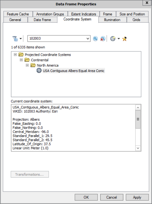
- Before we import anything, lets set the projection of the dataframe to an equal area projection so that we can accurately visualize these within the context of dispersion.
- Right click in the white area and go to properties > Coordinate Systems and search for WKID: 102003
- Let’s next bring in the csv. Drag the csv file from the ArcCatalog panel into the dataframe.
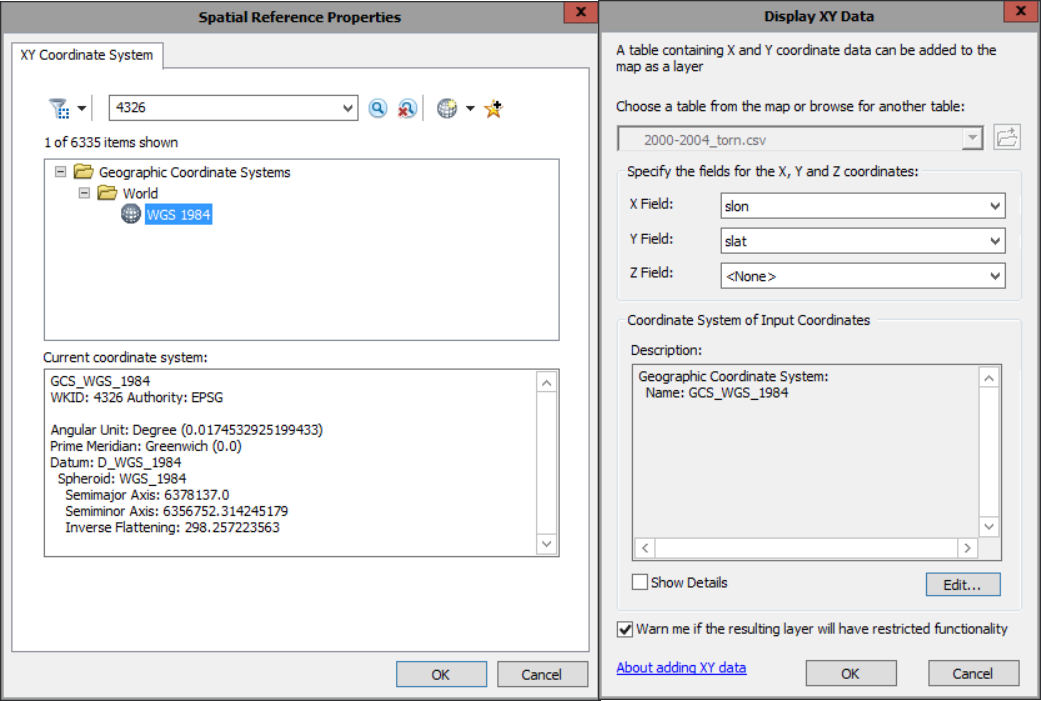
- Right click on the csv and “Display XY Data”.
- Set X Field to slon
- Set Y Field to slat, and then edit the coordinate system.
- Set the spatial reference of the data to WKID: 4326
- OK your way through the tool.
- Finally, as you might have noticed with the warnings, this layer has restricted functionality. To resolve this, we just need to export the data by right clicking on it and going to Data > Export
- Save All records
- Save the reference system as the data frame
- Save the output as a shapefile called Torn_yyyy_yyyy.shp
- Click yes to add the results to the window.
- Finally, remove everything from your dataframe with the exception of Torn_yyyy_yyyy.shp
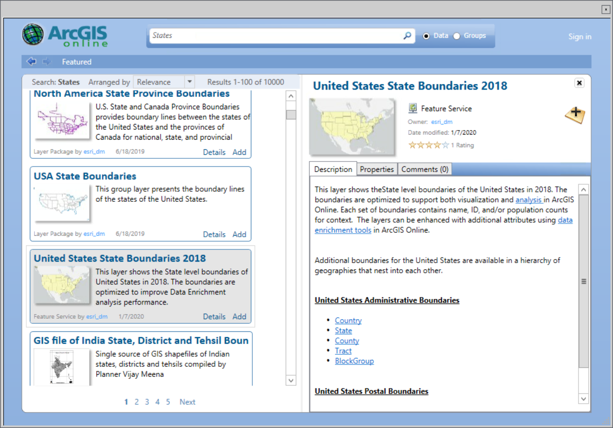
- Next add a state boundaries shapefile from your provider of choice.
- The quickest way to acquire this is to use the arrow dropdown next to add data and “Add Data from ArcGIS Online…”
- You will need to sign in to an ArcGIS account in the upper right hand corner.
- Search for “United States States”, and make sure the layer you add is a feature layer.
- Select the lower 48 states (and DC) from the layer that loads in, and then re-export the layer as lower48.shp.
- If this fails for some reason, you can grab state boundaries from TIGER.
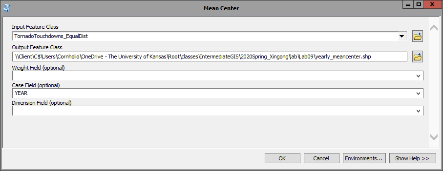
1) Open the Mean Center tool.
- In the Mean Center dialog box, select Torn_yyyy_yyyy.shp as your input feature class.
- name the output feature class Torn_yyyy_yyyy_mcy.shp.
- set the case field to yr.
2) Open the attribute table for Torn_yyyy_yyyy_mcy. Notice that you have n records, one for each year of data you imported. In order to use tracking analysis, the extension ArcMap uses to create videos, we need to create a new field, and populate it using Field Calculator to create a readable by the tool. We’ll assign a single day, for example, “7/1/1950” to represent 1950
- In the table options, Add Field to create a new field named TA_YEAR
- Set the type to Text
- Set the length to 32 byte
- Right-click on the newly created field and use the Field Calculator
- Enter the following expression:
"7/1/" & [yr]using VB Script.
- Enter the following expression:
3) Calculate monthly standard deviation ellipses using the Directional Distribution (Standard Deviational Ellipse) tool in the Spatial Statistics Tools -> Measuring Geographic Distributions toolbox. Afterwards, add the appropriated field for tracking analysis.
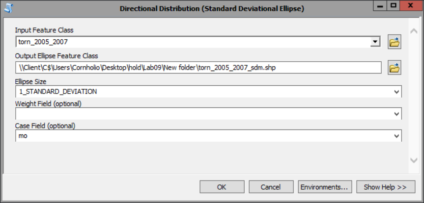
- Select Torn_yyyy_yyyy.shp as your input feature class.
- Name the output feature class Torn_yyyy_yyyy_sdm.shp
- leave the ellipse size to the default
- set the Case Field to mo
- Click OK.
- Add a new field named TA_MONTH (Text type, 32 byte length)
- assign the date (use the expression:
[mo] & “/1/05”for VB Script)
4) Create a temporal layer from the Torn_yyyy_yyyy_mcy points
- Activate the Tracking Analyst Extension and add it’s toolbar.
It might have been a while, where do you turn on extensions & add toolbars? (Hint: Customize > extensions & right click on the gray area in the > toolbar area)
- Leave the lower48 layer on and remove all the other layers
- Click on the Add Temporal Data wizard button
- You want to add a feature class or shapefile containing temporal data (first radio button) and click on the browse button to select Torn_yyyy_yyyy_mcy.shp as the input
- Select the appropriate date/time field (i.e. TA_YEAR) and click Next
- Specify the date & time format (M/d/yyyy) and click Next then Finish. A new “Temporal Layer” will be added to the data frame’s table of contents
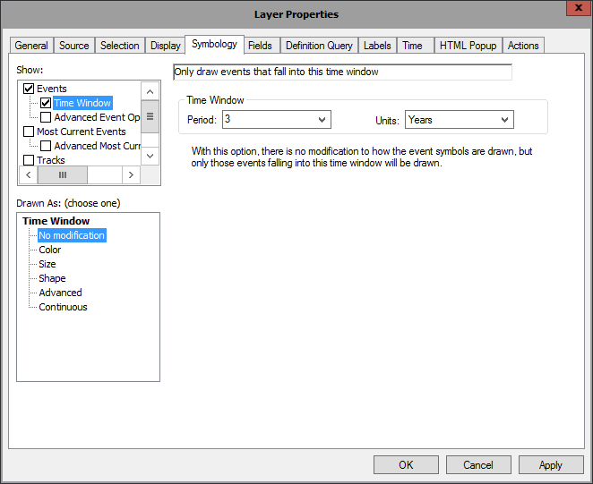
5) Modify the symbology of the temporal layer
- Right-click on the Temporal Layer and go to Properties
- notice the properties tabs are slightly different from those of a typical shapefile
- In the Symbology tab check the Time Window box in the Show: box under Events
- The number of periods is the number of intervals in the series, set as appropriate.
- For Torn_2005_2007_mcy.shp, the number of periods is 3 and the units are Years
- Click OK. You have set the temporal symbology (i.e., what symbols will display over time)
6) Visualize the temporal data
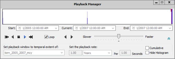
- Click on the Playback Manager button on the Tracking Analyst toolbar
- Hint: Hover over tools to see their name, remember?
- Click on Options and set the temporal extent to the temporal layer (Torn_yyyy_yyyy_mcy)
- Change the playback rate to 1.00 years per second
- Click play and watch the animation
- Write a film analysis detailing the evolution of the main character (Torn_yyyy_yyyy_mcy), with respect to the changing of the seasons.
- I kid…
7) Export the animation to a movie
- On the Tracking Analyst toolbar, go to Tracking Analyst -> Animation Tool
- Change the frame size width to 320 and be sure Maintain Aspect Ratio is selected. Set the output file to yourname_yearly_ttmov
- Click Generate.
- Go to Windows Explorer and launch your movie to make sure the animation was generated correctly.
- Answer question #1 on your answer sheet
1) Select tornado touchdowns within Kansas in 2005.
- Starting with lower48 and the Torn_yyyy_yyyy.shp, export the tornado touchdown data for 2004
- select by attributes, input layer Torn_yyyy_yyyy.shp, “YEAR” = ‘2005’, R-Click layer, Export Data…) and call it tt_KS_2005.shp, add it to the map
- Turn off the Torn_yyyy_yyyy and tt_KS_2005 layers temporarily and use the select tool to select Kansas (alternatively you can use the Select by attributes tool)
- Go to Selection > Select by Location, select features from tt_KS_2005 that intersect the features in lower48, and check Use selected features. It should inform you that there is one feature (Kansas State) selected.
- Click OK
- Turn the tt_KS_2005 layer back on to verify that only touchdown points for the year 2005 in Kansas are highlighted
2) Using the Average Nearest Neighbor tool in the Spatial Statistics Tools | Analyzing Patterns, calculate the Nearest Neighbor Index for Kansas in 2005.
- Input feature class: tt_KS_2005, use Euclidean distance and check Generate Report
- To see the report, open the ‘NearestNeighbor_Result.html’ in the Results window
- Click OK and fill in the appropriate information in the table (question #2 on the answer sheet)
3) Calculate Nearest Indices for Washington (the state) and Alabama in 2005
- Repeat parts of step 1 and step 2 above for both Washington and Alabama
- Fill in the table in question #2 and answer question #3 on the answer sheet
4) Calculating Nearest Neighbor Indices for two months (May and November) across the US in 2007
- Select the touchdown points that occurred in May of 2007 (select by attributes) and export data, naming the output tt_May07
- Do the same for November and name the exported dataset appropriately
- Repeat step 2 to calculate the NNI for the two months
- Fill in the table in question #2 on the answer sheet
5) Calculate the total area of the 48 conterminous states and DC
- Open the attribute table for the lower48 shapefile
- Add a new field named AreaSQM. Make it type Float
- Right-click on the AreaSQM field and click on Calculate Geometry
- Make the property Area and use coordinate system of the data source. Keep the units as square meters and click OK
- R-Click on the AreaSQM field, click on Statistics, and note the Sum. Answer question #4 on your answer sheet.
6) Use the total area to calculate NNI of the tornado touchdowns in May and November of 2007
- Repeat step 2 but include the total area figure in the area box.
- To make this easier, select the value from the statistics window and hit CTRL-C to copy the text to the clipboard. Then click on the Area field in the Nearest Neighbor window and use CTRL-V to paste the number).
- Fill in the results in the table in question #5 on your answer sheet.
7) Calculate the Nearest Neighbor Indices again, this time using using each region’s respective area.
- Repeat the above steps for Nearest neighbor analysis.
- You can copy the value from the attribute table and paste it into the dialog box).
- Fill in the rest of the table in question #5
8) Using what you’ve learned, answer questions 6 & 7 on your answer sheet.
Submit your final answer sheet to blackboard.