Lab 07 - Siting a New School with Model Builder and Fungus weight
In ArcGIS, we can build a model, based on a flow of data through a series of GIS operations, to arrive at a desired end. We will be using Model Builder to create a suitability layer for school siting in Stowe, Vermont in an automated way (yes, this was the same lab from intro class, we’re going to create the model this time). In essence, we will be setting up a diagram in Model Builder that will calculate the suitability raster with one click. Using Model Builder is helpful in situations where similar operations need to be applied in a programmatic way.
Lab 7: Answer Sheet
Name:
Part 1: Siting a New School with Model Builder:
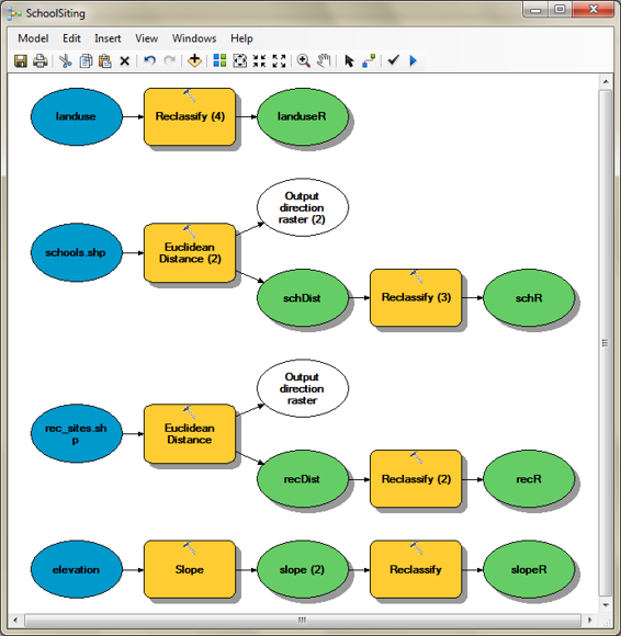
Question 1: In your model window, go to Model | Export | To Graphic…. Export the model as a png file and call it yournameLab7_1.png (i.e. rooseveltLab7_1.png). Double-check the image file to make sure all the objects are readable and paste it below.
Question 2: Total area of land with suitability 8.5 or greater for new school: m2
Part 2: Fungal Dispersion
Question 3: Using your model, complete the table below. For each city, put an “X” in the box that corresponds to the first month the fungus “invaded” the city.
| CITY | Jan | Feb | Mar | April | May | June | July |
|---|---|---|---|---|---|---|---|
| Selma, AL | |||||||
| Montgomery, AL | |||||||
| Pensacola, FL | |||||||
| Clarksdale, MS | |||||||
| Enterprise, AL | |||||||
| Lawrenceburg, TN | |||||||
| Albany, GA | |||||||
| Starkville, MS | |||||||
| Greenwood, SC | |||||||
| St. Augustine, FL | |||||||
| Natchez, MS | |||||||
| Wright, FL | |||||||
| Eufaula, AL | |||||||
| Mobile, AL |
Question 4: You must do one of the two following (do the other for extra credit!)
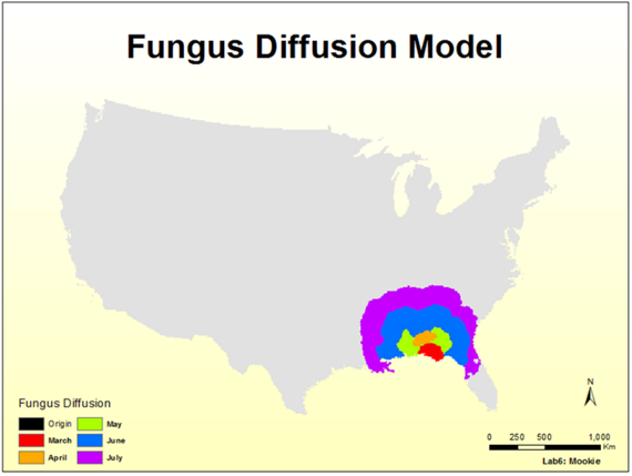
- Work on the Layout View to create a composite map showing the area invaded by the fungus by the end of each month. In other words, the legend should have 6 possible values, one for each month (including the origin). Make the colors contrasting enough so that you can see the difference between them. Be sure to add your name, a title and a legend. (See the sample map for a guide).
-or-
- Submit an image of an equivalent model needed to reproduce the output of the second part of the lab Save your map as a .PNG file using the Export map option of the File menu. Save it in your local lab07/Part2 folder and call it fungus_yourname.png
Upload the answers to the questions above along with your images to blackboard. The images are worth roughtly 1/2 of this labs grade so don’t forget to include them!
| Relevant part | Data Name | Description |
|---|---|---|
| Part 1 | elevation | Raster dataset of the elevation of the area |
| Part 1 | landuse | Raster dataset of the landuse types over the area |
| Part 1 | rec_sites | Feature dataset displaying point locations of recreation sites |
| Part 1 | schools | Feature dataset displaying point locations of existing schools |
| Part 2 | pre_01, pre_02, etc. | Monthly Precipitation (mm) for January through July |
| Part 2 | us48mask | Grid of 1s for states and no data for other cells |
| Part 2 | fungus_origin | Origin of Fungus in Panama City, FL |
| Part 2 | us48cities | Location of Major Cities in U.S. (Vector Data Model) |
NOTE: Each raster is in the Albers equal area map projection with a 10,000m x 10,000m cell size.
- Create a new toolbox (Lab7Tools), and a new model (SchoolSiting) in that toolbox.
- R-click on your lab07/Part1 folder and create a new toolbox.
- Name the new toolbox Lab7Tools.tbx.
- R-click on the toolbox and create a new model.
- Rename the new Model (R-click/slow-click | Rename) to SchoolSiting.
- Set up the Model Properties by going to Model | Model Properties
- Under the Environments tab, check the boxes for Processing Extent | Extent and for Raster Analysis | Cell Size
- Click the Values… button.
- Click the down arrows for each of the settings and make the Extent the same as the landuse raster in your data folder, and the Cell Size the same as elevation.
- Click OK on the Environment Settings.
- Click OK on the SchoolSiting Properties Window.
You will create a workflow diagram in the Model window that will show all the steps and operations/tools needed to get the suitable school sites. We start the process by dragging tools from ArcToolbox into the Model window to perform a specific operation.
- Set up your screen so you can see both ArcToolbox and the model window at the same time.
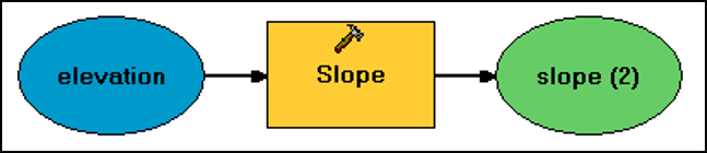
- Add the slope tool by finding it under ArcToolbox (Spatial Analyst Tools | Surface) and then dragging it onto the model window.
- Double click on the slope tool. The slope dialog will open, and will look familiar.
- Set the input to the elevation raster (from your data folder), and set the output to slope and make sure it is saved in the output folder in the Lab 7 folder. Leave other parameters to their defaults.
- Click OK. You will see the diagram objects become colored. You now have a very simple model.
- Next, add the Euclidean (straight line) distance tool (Spatial Analyst Tools | Distance | Euclidean Distance) to create a distance layer from rec_sites.
- Set the Input to rec_sites (from your data folder), the Output to recDist in your output folder, and the Cell Size to 30. You don’t need a Maximum distance or a direction Raster.
- Click OK. Notice that an empty diagram object is there for direction raster. Since it is blank, it will be ignored, so we will leave it alone.
- Add and set up another straight line distance tool to calculate distance from schools (call the output schDist).
- Save your Model (Model | Save).
- Click the Run button. Check in ArcCatalog to make sure that these three layers are calculated correctly and saved in your output folder.
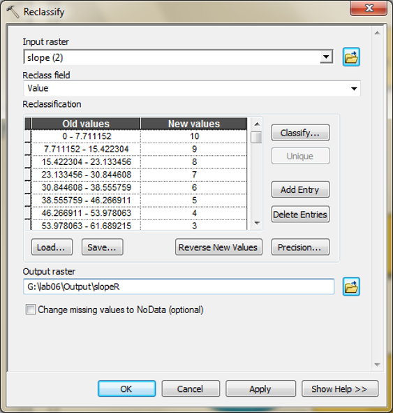
- Add a Reclassify tool (Spatial Analyst Tools | Reclass | Reclassify) to the Model window to reclassify the slope raster.
- Double click on the Reclassify tool in the Model window. Select slope as the input layer.
- This time, select the input layer from the dropdown in this dialog window, which shows the layers that are part of the model (We do this so that it will perform this next step from what we calculated in the previous one. In other words, it maintains a flow within the model).
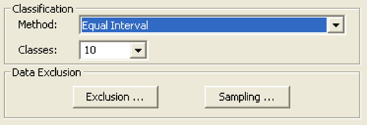
- In order to create the new classes for the slope layer, click on the Classify button, select the Equal Interval Method and 10 classes. Click OK.
- It is preferable that the new school site be located on relatively flat ground. You will reclassify the slope layer, giving a value of 10 to the most suitable slopes (those with the lowest angle of slope) and 1 to the least suitable slopes (those with the steepest angle of slope). Click on the Reverse New Values button so the lowest slopes get a value of ten and the steepest slopes a value of 1.
- Name the output raster layer as slopeR and click OK.
- Add a new Reclassify tool and double click on it.
- Select the RecDist layer as the input raster from the dropdown.
- Reclassify distance to recreation sites raster (recDist) into 10 classes with new values from 1 to 10 using Equal Interval classification method. The school should be located near recreational facilities. You will reclassify this dataset, giving a value of 10 to areas closest to recreation sites (the most suitable locations), giving a value of 1 to areas far from recreation sites (the least suitable locations), and ranking the values in between.
- Name the output raster layer as recR and click OK.
- Add a third Reclassify tool and double click on it.
- Select the SchDist layer as the input raster from the dropdown.
- Reclassify distance to schools raster (schD) into 10 classes with new values from 1 to 10 using Equal Interval classification method. It is necessary to locate the new school away from existing schools in order to avoid encroaching on their catchment areas. You will reclassify the distance to schools layer, giving a value of 10 to areas away from existing schools (the most suitable locations), giving a value of 1 to areas near existing schools (least suitable locations), and ranking the values in between.
- Name the output raster layer schR and click OK.
- Save your Model.
- Add and set up a fourth Reclassify tool in order to reclassify the landuse raster.
- Select ‘LANDUSE’ as the ‘Reclass field’ using the dropdown menu.
- Use the following table to assign the new values to each of the land use categories:
| Landuse type | Score |
|---|---|
| Agriculture | 10 |
| Barren land | 6 |
| Brush/Transitional | 5 |
| Built up | 3 |
| Forest | 4 |
| Water | NoData |
| Wetlands | NoData |
- Call the output landuseR.
- Click OK and Save your Model.
- After all four reclassify tools are correctly established in the model, click Run again and check your output folder to make sure everything was calculated correctly.
- With all of our standardized layers, we are ready to calculate our suitability raster. Add a Raster Calculator Tool (Spatial Analyst Tools | Map Algebra | Raster Calculator) to the Model window.
- Double click on this tool to set up the parameters.
- Create an expression to weight each factor using the table below.
| Layer | Weight |
|---|---|
| Reclass of distance to recreation sites (recR) | 0.5 |
| Reclass of distance to schools (schR) | 0.25 |
| Reclass of landuse (landuseR) | 0.125 |
| Reclass of slope (slopeR) | 0.125 |
Learning Objectives:
This lab will introduce you to the concept of modeling a diffusion process using friction surfaces that change in space and time. Your goal is to model the diffusion of a fungus from its introduction at a seaport in Panama City, FL on January 1, 1989 throughout seven months of the calendar year (i.e., January through July).
- Add all 7 precipitation grids, fungus_origin, us48mask, and us48cities.
- Go to Geoprocessing | Environments… and under Raster Analysis set mask to us48mask.
- Under Processing Extent set the Extent to Same as layer us48mask.
- Set the current workspace and scratch workspace to your lab07/Part2 folder.
- Rearrange (if necessary) the precipitation raster layers in chronological order.
- Save your project as lab7lastname.mxd (e.g.: lab7washington.mxd).
You will now model a diffusion process across a changing velocity surface. You will implement the time steps sequentially. The procedure for modeling diffusion across a dynamically changing environment involves the following steps:
- Establish the origin (for the first run, it will be fungus_origin).
- **Reclassify** the Nth month of precipitation to a velocity grid (units of meters per day) based on velocity for each precipitation range.
- Identify the maximum value of precipitation for that month.
- Hint: The table of contents shows the range at a glance.
- Use the Reclassify tool ( ArcToolbox | Spatial Analyst Tools | Reclass | Reclassify) to reclassify the precipitation for that month (e.g: pre_01 for January)into a friction rate according to the following assumption about the disruption speeds.
* Name the output velocity_nn. * If writing out the table each time is too tedious for you, you can click “Save…” and save the reclassification look-up table as a table named diff_rate which you can reuse.Precipitation Amount Rate of Movement < 100 mm/month 0m/day 100 - 200mm/month 4000m/day 200mm/month and greater 7000m/day 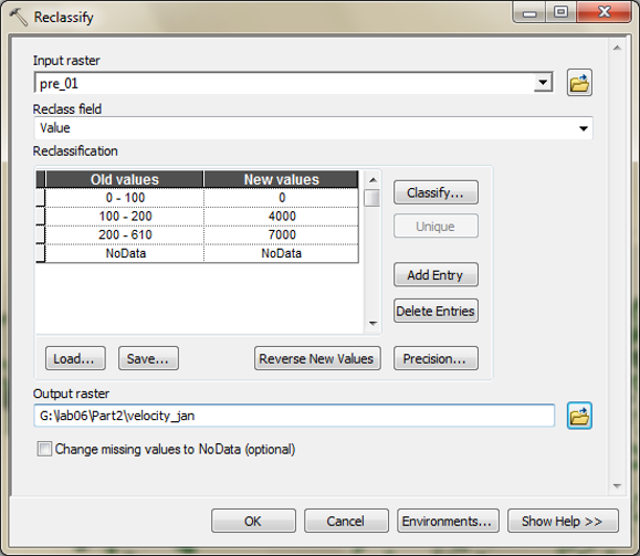
- Identify the maximum value of precipitation for that month.
- Create a Time per Unit Distance grid (days per meter).
- Using the Raster Calculator, create the following expression: 1 / Float(“velocity_nn”)
- Name the output friction_nn.tif
- Model the diffusion possible diffusion range for the Nth month by using the **Cost Distance** (ArcToolbox | Spatial Analyst Tools | Distance | Cost Distance) operation. Name the output diffuse_nn.tif
- For example: this will change as you go
- Input Raster: fungus_origin
- Input Cost raster: friction_01
- Output Distance Raster: diffuse_01.tif
- For example: this will change as you go
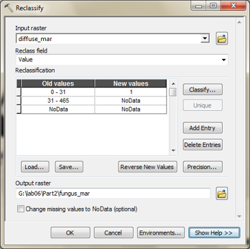
- Create a new origin raster by reclassifying the travel time raster (diffuse_nn) from the previous step based on the number of days in the month, again using the **Reclassify** tool. Your goal is to set all values less than or equal to the number of days in a particular month to a value of 1, and all other values to no data (make sure you set proper maximum value for each month based on the number of days). Name the output raster as fungus_nn.tif (e.g., fungus_01.tif).
Month Days Jan 31 Feb 28 Mar 31 Apr 30 May 31 Jun 30 Jly 31 - Redo these processes for each successive month using the new fungus distribution (e.g., fungus_01) as your new origin, and repeat this until you have modeled fungus diffusion through July (07).
- Save your map as Lab7yourname.mxd
- Complete questions #3 – #4 on the assignment sheet.