Lab 05 - Model Builder

As you have likely noticed, the process of delineating a lake follows a predictable workflow that could easily be automated, and because time is money, it would behoove us to create a script one could run which would create the needed outputs for us without all the tedious clicking and typing that would otherwise have to occur. Fortunately, ArcGIS has a mode, ModelBuilder, which enables us to visually create a workflow to connect our data to a series of operations without the need to actually code in python. To do this effectively, we need to modify our process somewhat, so the first part of this lab will walk us through the steps needed to perform this analysis on a single year, and part 2 will introduce the model builder interface and how this process can be automated and applied to each year we downloaded in lab 1. By the end of this lab you should have a firm grasp on the local, focal and zonal operations we need to use to create the lake, and how model builder can be used in numerous applications to speed up your workflows.

Submit an image of both your analysis and a screenshot of your model to blackboard. Then submit your screenshot to the Google Spreadsheet.

• Open ArcMap and make sure that the Spatial Analyst extension is activated, and overwriting files is enabled.
  • Customize > Extensions & ArcMap options.
• Rename the default data frame to Base Data and add in the AOI, Bands 2 and 4, and the MTL file for each year.
• To force our model to calculate everything using a consistent grid size, change the geoprocessing > Environments settings to the following:
  • Workspace: Set both the Current workspace and Scratch workspaces to your lab05 folder.
  • Processing Extent: Use the folder icon and point it to your AOI shapefile. Use the folder icon next to snap raster to select the elevation dataset.
  • Raster Analysis: Select As specified below and type in 30.
  • Click OK.

As you discovered in lab 4, the region group tool was useful in creating a raster we could use to select the desired areas. However, the region values were quasi-random. Although we could in theory make a program and so this will not work if we are attempting to create a programmatic workflow. We will instead use a “seed” and the cost distance tool to classify which of the NDWI zones we want.

• In the ArcCatalogue window right click on your basedata geodatabase and create a new feature class.
• Call the class LakeSeed and make it a point feature. Click next.
• Use the Layers box to select the correct projection. Click next until you reach the Field Names category.
• In the first empty Field Name box, type in VALUE and change the Data Type to Short Integer. In the field properties you can set the default value to 1. Click Finish. The layer should be added to your window.
• On the Editor toolbar, click Editor > Start Editing.
• In the Create Features window, click LakeSeed and choose the point tool.
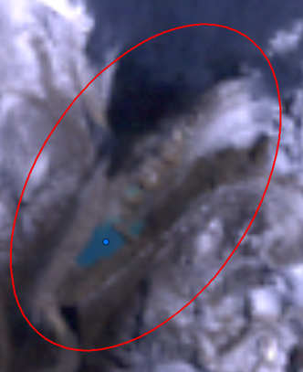
• Create a single feature that will “intersect” all lake layers through time, so the center of the smallest lake extent is best.
• When finished, click editor > stop editing and save edits.
  

Recall from lab 2 that this expression needs appropriate parenthesis and the Float() attribute. However, we want to reverse the expression here so that we want to classify as a lake has a 0 value, and everything else has a value of 1. This way we can use the cost distance tool to traverse all connected lake pixels without inuring a cost.

• Hint: My expression looks like
  (Float(“1995\LT05_…_B2.TIF” - “1995\LT05_…_B4.TIF”) / Float(“1995\LT05_…_B2.TIF” + “1995\LT05_…_B4.TIF”)) <= 0.3
• Call the output NDWI_yyyy.tif.

• Use the search bar to find the Cost Distance tool.
• The source data is the LakeSeed.
• The input cost raster is the NDWI_yyyy.tif layer.
• Save the output as Cost_yyyy.tif.
• We want just the lake, so use raster calculator and get just the areas with 0 cost
  • Hint: “Cost_yyyy.tif” ==0
  • Save the raster as Lake_yyyy.tif

(as per lab 3)

• Using the Focal statistics tool, calculate the focal minimum using a rectangular 3x3 grid
• The input should be the Lake_yyyy.tif layer
• Save the output Lake_yyyy_Fmin.tif
• Using raster calculator, subtract the focal min raster from the lake classification raster to get just the boundary.
• “1995\Lake_yyyy.tif” - “1995\Lake_yyyy_Fmin.tif”
• Save the output of the map as lakeEdge_yyyy.tif

As per lab 4 we will use zonal statistics as table and our newly created zone to calculate the (insert statistic here) value of the elevation data.

• Use the lake boundary (lakeEdge_1995.tif) as our zonal definition
• We want the statistics from the elevation data, so that goes in the “Input Value Raster” box
• Choose a statistic, I chose maximum but feel free to explore other options
• Save the output as …LakeBoundary_ZonalStat

Also from lab 4 use the reclass by table function (spatial analyst) to reclassify the lake_1995 raster into a lake surface raster.

• Your input raster is Lake_1995.
• Your remap table is the table created from zonal statistics as table (LakeBoundary_ZonalStat)
• The From, to, and output value should fill in automagically, but in case they don’t think about what you are trying to accomplish.
  • The from and to value need to match, you are essentially joining tables together here, so both need to be VALUE
  • The Output field is the value that you are reclassifying to, so this should be MAX
  • Save the output as LakeSurface_yyyy.tif

We need just the lake elevations, and given the tools shown so far we could accomplish that by multiplying them with the Lake_1995 raster using raster calculator (to set the values we no longer want to 0), and then setting the 0 values to NoData. We can do this in 1 step through raster calculator using the Set Null function. The Set Null(,) function takes two arguments, a mask which sets the values to null and a raster with the values to set otherwise.

Hint: SetNull(“Lake_yyyy” ==0, “LakeSurface_yyyy.tif”)

• Save the output raster as LakeSurface

• Subtract the DEM from the Lake Surface using the raster calculator tool
  • Save the output as LakeVolume.tif
• Use the Add field tool (data management) to create a new field
  • Call it volume
• Use the Calculate Field tool to calculate the volume of each cell
  • Hint: Depth(Value) * area (30*30) * Count
• Use the summery table to create a table of volume (an optional step, otherwise just know that you’ll need to sum the field yourself each time.

This process was time consuming, and the only thing that changes in this workflow (once we’ve chosen a place to analyses), is the input bands. This repetitious task is best completed using a function. In ArcMap, functions can take the form of tools, and the visual programming interface called Model Builder.

• In your lab folder in the ArcCatalog pane, create a new File Geodatabase
• In that same lab folder, Right click and create a new > toolbox. Name it LakeVolumeAnalysis.tbx
• Right click on that toolbox and create a new > model.
• A blank Model window will appear. Take a moment to explore the tools. You can go to ArcGIS Desktop Help to find more information about each of the tools.
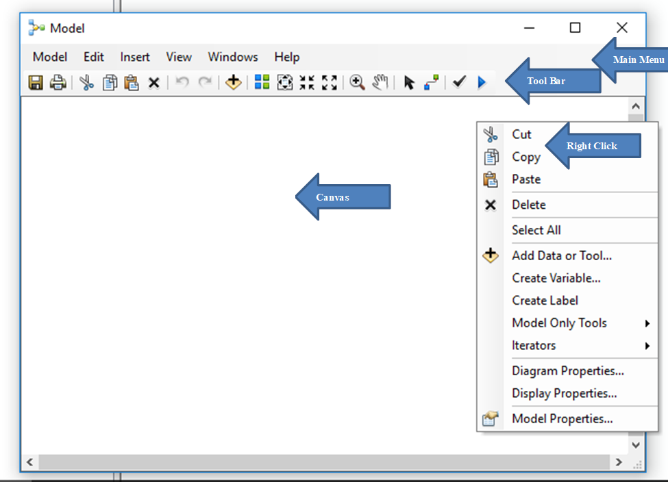
• Close the Model window.
• Right click on the model and
  • In the general tab rename the model LakeVolumeForAYear
• Re-open the Model by R-clicking and selecting Edit…
• Set up the Model Properties by going to Model | Model Properties
• Under the Environments tab, check the boxes for Processing Extent | Extent and for Raster Analysis | Cell Size, and for Workspace
• Click the Values… button, and set the values as in part 1A
• Remove all layers from the map

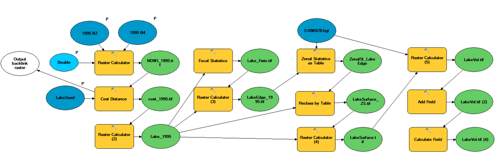
You will create a workflow diagram in the Model window that will show all the steps and operations/tools needed to delineate the sea level change. We start the process by dragging tools from ArcToolbox into the Model window to perform a specific operation.

• Open ArcToolbox and set up your model window and ArcMap window so that you can see both ArcToolbox and the model window at the same time.
• Use the add data button to add in the band 2 and band 4 rasters
• Right click on the resulting oval and rename it to Band 2 and 4 respectively
• Right click on it and make it a parameter by checking Model Parameter option from its popup menu (right-click). The letter P appears beside the variable, indicating it is a model parameter.
• Insert a new variable with insert > create variable
  • Select Double
• Double click on it and give it a default value of 0.3
• Right click on it and make it a parameter as well.
• Use the search function to drag in the raster calculator tool from ArcCatalog into the model builder canvas
• Double click on the raster calculator tool and fill it out as appropriate using the steps above.
  • Make sure you use the drop downs to populate the raster calculator, pointing at the data is not appropriate here.
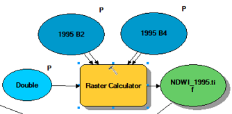
  • Hint: My expression looks like (Float("%1995 B2%" - “%1995 B4%") / Float("%1995 B2%” + “%1995 B4%")) <= float(%Double%)
  • Name the output NDWI.tif
• The bubbles should color themselves in if you entered everything in correctly. This means that the tools executed successfully, but be careful. Just because it ran doesn’t mean it is right. Your model should now look like so:

Build the rest of the workflow as defined above by dragging in tools using the same process. A few places of minor note. When you use functions in modelbuilder, you will most often want to use the layers which have a recycle symbol next to them. These are model variables, and in tool prompts they are bracketed by % signs. So for example when you add the Set Null(,) function, it should be parameterized as follows:SetNull("%Lake_1995%” ==0, “%LakeSurface_yyyy.tif%")

Your final model should look like this:
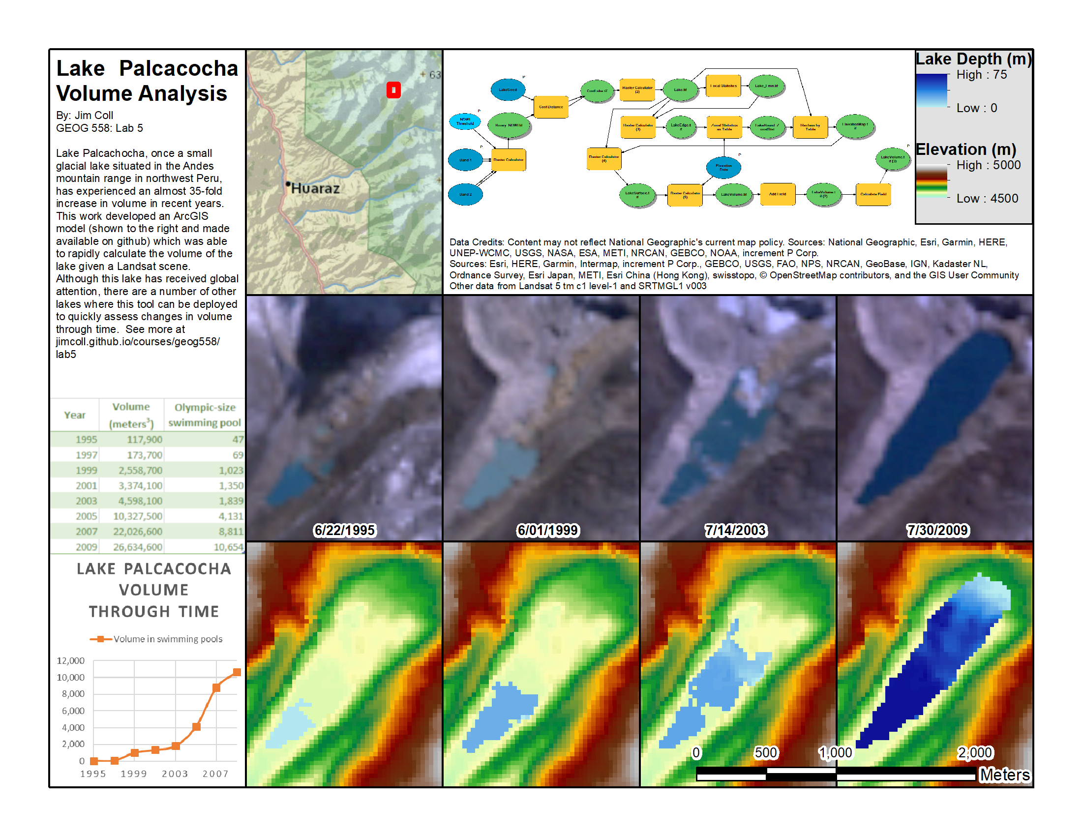
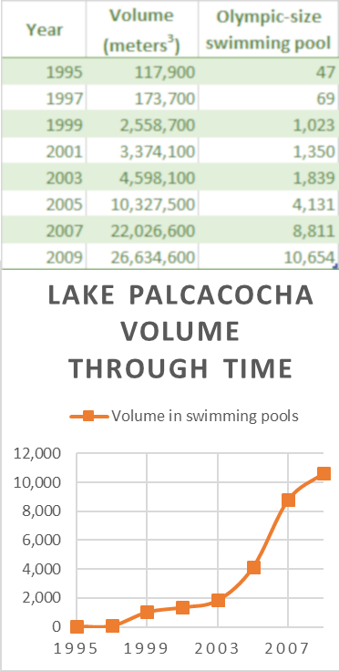
Once the model is up and running, you can feed it the appropriate bands for each year to rapidly perform a lake volume analysis. Create a chart/table of the lake volume change over time, mine looks like so:
Finally, submit an image of both your analysis and your model to blackboard. Create a final map of this lake analysis. This will be the last time we look at this lake this semester, so spend some time saying your goodbyes. You’ll also share your map in the Google Spreadsheet (linked on bb) so we can critique them after spring break. Feel free to use mine as inspiration.