Lab 10 - Spatial Interpolation
When we deal with spatial analysis, one of the problems we have is getting data we collect in the field into a form we can analyze. Most field data are collected at discrete points (e.g., rain gages, GPS point collection, address points, ect.). There are several interpolation methods that allow us to take this point data and make it into a continuous surface. We will look at the Inverted Distance Weighting and Kriging methods in this lab.
Scenario:
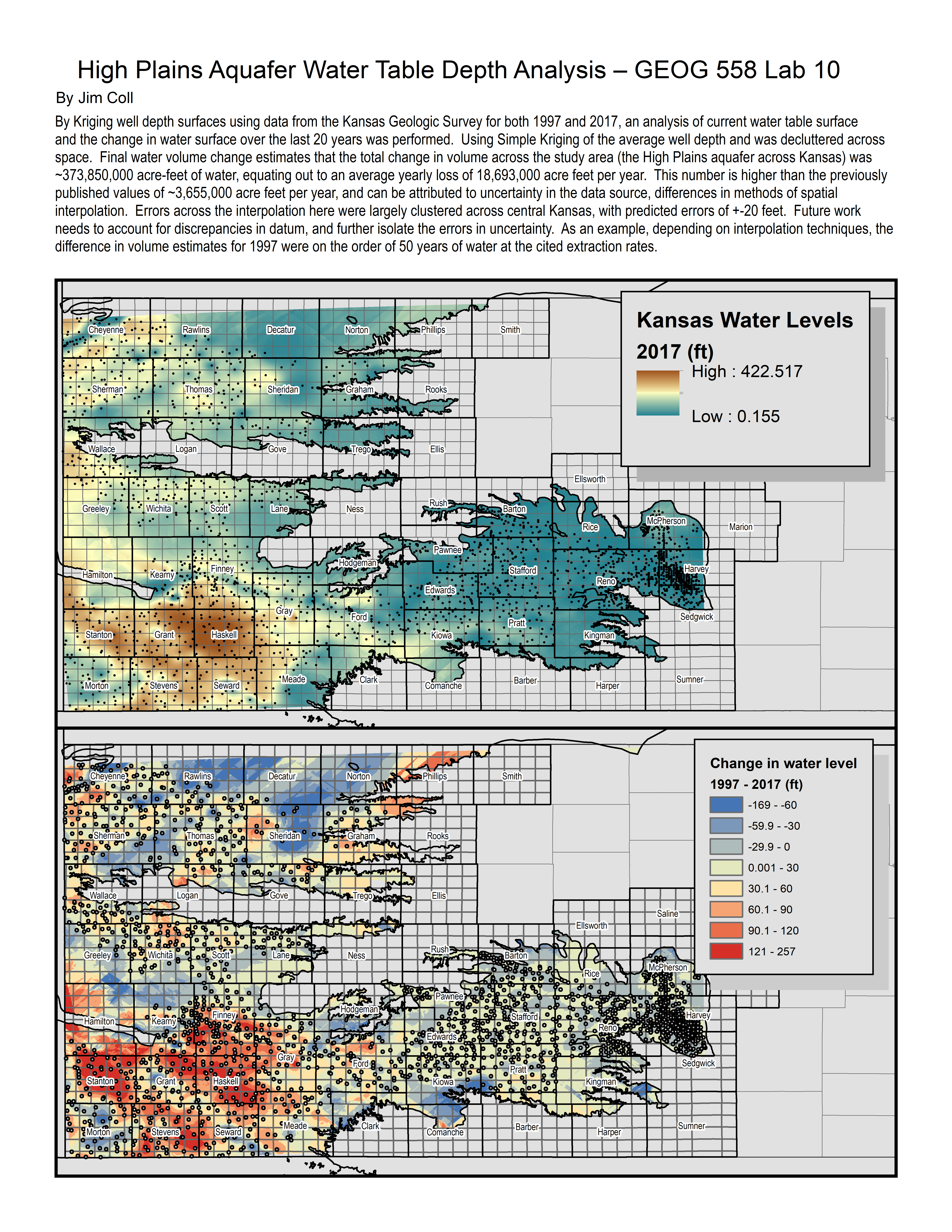
You have been hired by KGS to perform an analysis of water level in the High Plains Aquifer in Kansas. They have provided you with 2 shapefiles containing min, mean, and max water level depths from the surface for 1997 and 2017. Your job is to perform a volume comparison. You will need to interpolate a surface representing the water table elevation for each time period and determine the volume gained or lost over the 20-year period, create a map describing the status and change of the water table in Kansas, and a short report of your findings.
Outline:
Lab 10: Answer Sheet
Question 1:
What was your regression function?
Question 2:
What is the interpretation of your regression function?
Question 3:
What was your highest prediction standard error (hint: right click on the GA layer and “Change output to predicted Standard Error”)? How does this error compare with the distribution of the well heads?
Question 4:
Subtract the two 1997 surfaces. What is the difference in volume between the two interpolation methods. Given that we extract ~3,655,000 acre-feet of water a year, how important is the interpolation method in determining the change in volume?
Question 5:
Pick one of the interpolations and submit your report below. This might include some or all of the following elements.
- A “Current” depth to water level map (example from Brownie Wilson of KGS below)
- A difference map describing the change in water level over the time period
- A short (1-2 paragraph) interpretation of the outcomes. This should address common questions an employer might ask including an interpretation of the data, how the map was created, a statement of accuracy, and potential sources of error.
An example of how I might approach this question:
| Data Name | Description |
|---|---|
| HPWells_1997.shp | Well depths for Kansas within the High Plains Aquifer from 1997 |
| HPWells_2017.shp | Well depths for Kansas within the High Planes Aquifer from 2017 |
| SelectedStates.shp | Boundaries for Kansas, Nebraska, Colorado |
| KSCounties.shp | Kansas counties from the 2010 TIGER database |
| KSPLSSSections.shp | Kansas PLSS Section shapefile |
| HPBounds_2010.shp | Outer boundary for the High Plains Aquifer |
| smalldata.zip | A subset of the data for Kansas Groundwater Management District 4 |
Interpolating surfaces can be one of the more processing intensive operations. As an alternative if you are in a processing limited environment feel free to perform the lab using the “smalldata” folder in place of the full database. I have subset the original assignment to the 6 counties that comprise the Kansas groundwater management district 4.
1) Getting started
- Add the data into ArcMap and examine it’s properties.
- We will use the Geostatistical Analyst feature in ArcMap. There are many, many features of this tool that we will not explore here. You can use the ArcMap help system or Google “Using ArcGIS Geostatistical Analyst” online to explore this tool beyond what we will do here.
- If necessary, activate the Geostatistical Analyst (Customize | Extensions)
- Add the Geostatistical Analyst toolbar (Customize | Toolbars | Geostatistical Analyst)
2) Interpolating a surface using IDW
- Go to Geostatistical Analyst | Geostatistical Wizard
- Highlight Inverse Distance Weighting
- Select your Source Data (A well shapefile)
- We want to model a water surface, so make your Data Field (I use avg depth)
- Click Next
- If a “Handing Coincidental Samples” prompt pops up, decide how you would like to handle this occurrence. Since I prefer “worst case” scenarios, I choose “Use Maximum”. Once you’ve chosen, click next.
- This next window shows you how water levels will be modeled, but in a graphic form. Take a look at the help file for the statistical wizard to determine how the various inputs affect the statistic performed. ArcMap is nice enough to include a power optimization button under general properties. Go ahead and click that button. I also want to include more samples in my interpolation so change maximum neighbors to 25 and minimum neighbors to 7.
- The next page shows you the cross validation of your surface. This means that they take a point out of the prediction and compare it to the surface it would otherwise have been created without using it. When presenting results, most publications generally eschew printing the nuances of how they ran an interpolation tool in favor of reporting the regression function. Answer questions 1 and 2 below. When you are done click finish.
- The grid that the geostatistical wizard spits out is a format specific to the interpolation tools and is not easily manipulated as you have grown used to. Export it as a raster by R-clicking on the layer and going to Data | Export to Raster…
- Change the cell size to 500 and set the output raster to save it as IDWYYYY in your lab10 folder
3) Interpolating a surface via Kriging
Quick Kriging refresher here: https://gisgeography.com/kriging-interpolation-prediction/
- Go to Geostatistical Analyst | Geostatistical Wizard and choose Kriging / CoKriging
- Make sure your type of Kriging is set to Simple Kriging and Normal Score, and make sure the Output Type is Prediction
- Click Next
- This next window is unique to Normal scores, walking you through the normalization parameters. ArcMap does all the heavy lifting for you so take note of the parameters, look at the QQ plot, and then click Next
- Again, the modeling window includes an “Optimize model” button, click that and then click Next
- This visualization in the next window again shows the graphical representation of the interpolated surface in a graphic form. Click on the inset map to move the cross hairs to different portions of the aquifer. The circle around the cross hairs shows which area the model will take into account for that location. Leave all on this window to the set defaults and click Next
- This next window shows you the model and the Prediction Errors. You can save this validation result to a .dbf file (or a table in a shape file) that you can open in Excel, which may have a helpful feature, depending on your purposes.
- Click Finish
- Click OK on the Output Layer Information window and export the layer to a rater as above, using a name similar to KGYYYY
- Answer questions 3 below.
4) Clip the rasters to the extent of the Aquifer
Hint: clip tool… make sure you use the check box
5) Calculate Water volume difference between the two interpolation methods
- Hint: raster calculator…
- If you don’t have an attribute table, you will need to do the following:
- Use Raster Calculator to first turn the raster into an integer while keeping some of our calulated presision.
- Hint:
Int("KI1997Diff.tif" * 1000)
- Hint:
- Use the Build Raster Attribute table tool to generate the attribute table
- Create a new field called Volume, make it a float.
- Calculate volume using
((Value/1000)/3.28084)*Count*500*500 - Answer question 4
6) Pick an interpolation method and interpolate 2017 data using the same methods and parameters as above. Repeat steps 4 and 5 and answer question 5 on the sheet.