Lab 03 - Focal Operations
This lab will use neighborhood operators (i.e. focal operators) to examine an elevation surface, remove errors in a DEM, analyze wind exposure, and delineate the edge of our lake classified in Lab 2. In the first part, you will learn how to bring an ASCII into Arc as a grid and confirm your understanding of focal statistics. In the second, you will use the slope tool and focal statistics to blur out errors in the DEM and examine how changing the window results in a changing image. In Part 3, you will perform a site suitability analysis for wind turbines using the slope, aspect, hillshade, and focal wedge tools. Finally, we will use focal erosion to isolate the edge of our lakes classified in Lab 2. You can do all of these parts within the same or separate mxd’s, but be sure to save often.
Outline:
| Relevant part | Data Name | Description |
|---|---|---|
| Part 1 | Test.txt | ASCII Grid with sample values |
| Part 2 | silvrsub_f | DEM for Silverton, CO (30m cell size, elevation in feet) |
| Part 3 | wnw | DEM of NW part of Watauga Cnty (30m cell size, elevation in feet) |
| Part 4 | BaseData | Data downloaded in the first lab |
| Part 4 | NDWI_3.tif | NDWI threshold maps you created in Lab 2 |
- Open ArcMap and make sure that the Spatial Analyst extension is activated.
- Name the default data frame to ASCII Grid.
- Change the workspace for the Spatial Analyst Tools by going to Geoprocessing > Environments…
- Under Workspace change the Current Workspace to your Lab3 folder.
- Rename the data frame named ASCII Grid.
- Inspect the ASCII Grid file test.txt using a text editor such as notepad. We will use this small raster file to visually verify the results of several focal operations.
- Open ArcToolbox and Select Conversion Tools | To Raster | ASCII to Raster tool.
- Set test.txt as the input file and save the output raster as test in your lab03\part01 folder.
- Leave the data type to default and Click OK.
- The test raster will be added to the Table of Contents automatically. You can ignore any projection warnings you receive when adding these rasters.
- Use the ArcToolbox | Spatial Analyst Tools | Neighborhood | Focal Statistics tool to answer Question #1.
hint #1: change your layer symbology to show unique values.
Question 1:
Use your test raster layer to run the following three FOCAL operations (with a rectangular neighborhood of 3 by 3, cell size 10) and fill in the respective grids:Focal Sum: test_sum:
Focal Maximum: test_max:
Focal Mean: test_mean:
Want to flex? You can label the rasters as shown below, and it’s good cartography practice. Useful tools: Raster to points/extract values to points, label placement and halos, field representation to round to two decimal places.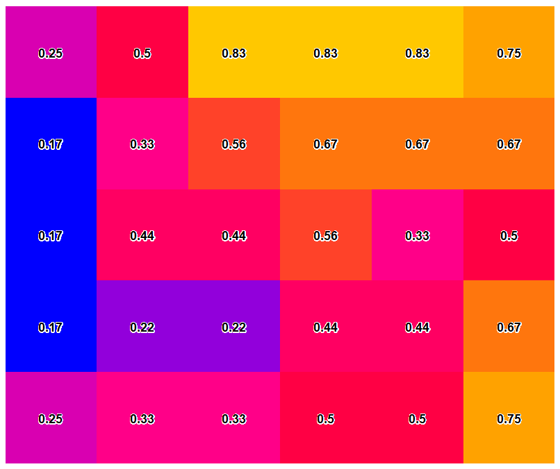
- Save your Arcmap document.
First let’s lay down the foundation.
- Insert and rename a data frame to DEM Error Removal.
- Add the silvrsub_f grid to the data frame.
- This surface was created in rectangular patches and then mosaiced together, but the artifacts of mosaicing are not readily visible by simply viewing the DEM.
- Since the height is in feet and the cell sizes are in meters, you should put everything into the same unit using a local operation (i.e., Raster Calculator).
Hint: 1 foot = 0.3048 meters.
- Save the output to your lab03\part02 folder as: silversub_m.
Let’s start by calculating the slope for the raster to more easily identify the artifacts.
- Open ArcToopbox | Spatial Analyst Tools | Surface | Slope, which is a focal operation we can use to find the linear artifacts in the silversub_m grid.
- In the slope dialog box, set the input raster as silversub_m.
- Leave the default values for output measurement and z factor.
- Save the output grid silver_slope in your lab03\part02 folder.
You should now be able to visually pick out the linear artifacts left from the mosaicing process. Using the measurement tool, determine the approximate size of the patches that were used to mosaic the image and answer Question #2 on your assignment sheet.
Now try to eliminate the artifacts by smoothing the surface of silversub_m before deriving the slope. Go to ArcToolbox | Spatial Analyst Tools | Neighborhood | Focal Statistics to compute the mean elevation value in a rectangular neighborhood of 3x3 cells and another of 7x7 cells.
- Use silversub_m as the input in both cases, making sure to name the output appropriately, something like silver3x3 and silver7x7.
- Derive the slopes of these new surfaces as in step 2, and be sure to name them appropriately, something like slope3x3 and slope7x7 respectively.
- Answer Question #3 on your assignment sheet.
First let’s lay down the foundation
- Insert a new dataframe and call it Wind Exposure Analysis.
- Add the wnw grid to the data frame.
This surface was created in rectangular patches and then mosaiced together, but the artifacts of mosaicing are not readily visible by simply viewing the DEM. Since the height is in feet and the cell sizes are in meters, you should put everything into the same unit, as was done in Part 2. Save the output to your lab03\part03 folder as: wnm_m
- Select the cells where the elevation in wnw_m is greater than or equal to 1000m by creating the following expression in the Raster Calculator: “wnw_m” >= 1000
- Make the output raster a permanent layer named GoodElevation
- Using Spatial Analyst, create a hillshade raster from your wnw_m DEM using the ArcToolbox | Spatial Analyst Tools | Surface | Hillshade tool
- Set wnw_m as your input surface, leave the default settings for azimuth and altitude, but set the Z factor to 3
- Save the output grid as hillshade in your lab03\part03 folder
Hiilshades are useful for providing geographic context, but can overwhelm data which kind of defeats the purpose of making a map. One way to fix this is mask out no data values in your output layer, and make it slightly transparent. We’ll do this a few times in this lab so remember this sequence
- Display GoodElevation on top of hillshade
- Set the color of the bad elevations (0’s) to hollow (no color) by:
- R-clicking on GoodElivation
- Select symbology tab
- Check box “display background value:”
- Proceed with: 0 symbol and selecting No Color.
- Change the Transparency value of GoodElivation to approximately 40%
- R-Click -> Properties under the Display tab
Answer Question #4 on your assignment sheet
- Calculate the aspect from wnw_m DEM using the ArcToolbox | Spatial Analyst Tools| Surface | Aspect tool
- Save the output grid as aspect in your lab03\part03 folder
- Notice the range of angles assigned to each direction in the table of contents. Aspect values begin at 0 at due north and increase clockwise.
- Using Raster Calculator, select the cells with an aspect between 225o and 315o. This will give us the westward facing slopes.
- That expression should look like (225 <= “aspect”) & (“aspect” <= 315)
- Make the output raster a layer named GoodAspect
- Display the GoodAspect on top of hillshade (set symbology like you did for GoodElivation) and verify that it represents the western slopes.
Answer Question #5 on your assignment sheet.
Create a neighbor mean raster of wnw_m using a FocalMean operation.
- ArcToolbox | Spatial Analyst Tools | Neighborhood | Focal Statistics with a wedge neighborhood (start angle 135, end angle 225, and a radius of 10 cells.
It is important to note here that the wedge neighborhood is measured differently than the aspect. The aspect measurement begins at 0 degrees due north and increases as we move clockwise. However, when computing a wedge neighborhood, we start at 0 degrees due east and increase as we move counterclockwise. Thus, the degree range here (135-225) represents the same degree range as indicated in the aspect range (225-315). This is simply due to inconsistencies in the way the ArcGIS software handles radial measurements. TODO: Add a nice image of this here.
- Save the output as WindMean10
- In Raster Calculator, select the cells whose elevations are higher than their neighbor mean (i.e., WindMean10)
- wnw_m > WindMean10
- Make the output a permanent raster named GoodWindExp10
- Display GoodWindExp10 on top of hillshade
- Using Raster Calculator, select the cells with good elevation (1’s), aspect (1’s), and wind exposure (1’s). Your expression can look like: (GoodElevation == 1) & (GoodAspect == 1) & (GoodWindExp10 == 1), or more simply GoodElevation * GoodAspect * GoodWindExp10.
- Make the output a permanent raster named GoodSites10.
- Use Raster Calculator, select the cells with good elevation (1’s), good aspect (1’s) and bad wind exposure (0’s) with the following expression: (GoodElevation == 1) & (GoodAspect == 1) & (GoodWindExp10 == 0).
- Make this a permanent raster named Blocked10, which indicate cells where the wind is blocked because of hills to the west.
- Answer questions #6 - #8 on your assignment sheet (you will need to repeat the steps above twice more using different radius values)
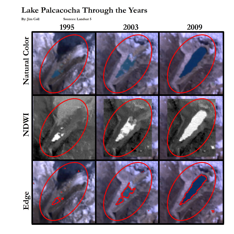
Open your Lab 2 Part 1 mxd or create a data frame/document. This document should have:
- AOI shapefile
- lake body classifications (…NDWI_#.TIF) )for 1995, 2003, and 2009.
- The RGB file for each year
- Using the Focal statistics tool, calculate the focal minimum using a rectangular 3x3 grid.
- The input should be the …_NDWI_3.TIF created in Lab 2.
- Save the output in the 1995 BaseData folder and name the output as …_NDWI_FMin.TIF.
- Using raster calculator, subtract the focal min raster from the lake classification raster using an expression such as: “1995\LT05_L1TP_…_NDWI_3.TIF” - “1995\LT05_L1TP_…_NDWI_FMin.TIF”.
- Save the output of the map as LT05_…_LakeBoundry.TIF.
- Move to layout view
- Set the page dimensions to 11 in x 11 (File, page and print setup)
- Use guides to set up 3 inch grids (click on the guides)
- Right click on the data frames to copy them
- Paste them in the frame and rename them to the appropriate place
- Text can be rotated in the properties
- To add grid lines, change the frame properties or using lines by adding the drawing toolbar (right click in the grey area as necessary)
- Finally, export your map