RS
Remote sensing is a course onto itself, but it’s worth introducing here as GIScience, GISystems, and remote sensing overlap more than they diverge. Remote sensing, as opposed to in-situ measurement, is the measurement of an object from a distance, most often a great distance.
This lab should provide you with the bulk of the background knowledge needed to dive further into the field of remote sensing. We’ll cover common terminology and technology, some basic applications, and cover how R can be used to perform common GIScience and remote sensing operations.
To start off, lets review some key vocabulary that often comes up when discussing remote sensing. These definitions are important when discussing concepts such as distortion and illumination angles but will only crop up sporadically.
- In physics, the nadir direction for a given location is the local vertical direction pointing in the direction the force of gravity acts at that location. In remote sensing this concept is, in essence, the point on a photo which is directly below the satellite. It’s opposite direction, zenith, refers to the direction directly opposed to gravity.
- Julian days are equivalent to Day of the Year, starting on January first of each year.
- Epoch time, also know as Unix time or POSIX time, is the number of seconds that have elapsed since January first, 1970 at midnight GMT/UTC, and is often used to indicate the timestamp of the data. (handy web converter)
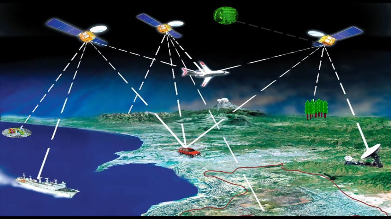
- Remote sensing data comes from instruments, or sensors, which in turn are housed aboard platforms, or satellites.
It’s difficult to learn about remote sensing without first recalling some basic physics. First, take a second and recall how eyesight and vision works, using the conceptual diagram below.
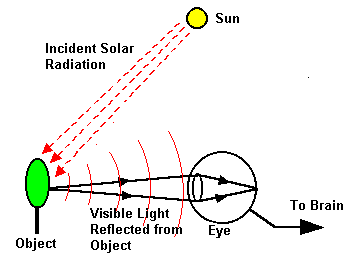
Remote sensing is the measurement of the electromagnetic spectrum. Energy (not necessarily in the visible spectrum) from a source, strikes the object, and then travels to the eye. We’ll break this down a little further. There are several different flavors of remote sensing, but the two most common ones are:
- Active sensing: A sensor or pair of instruments that both emit and receive measurements. Common examples of active remote sensing include ground penetrating radar, sonar, and LIDAR.
- Passive sensing: A sensor which only receives measurements. These are some of the most common forms of sensors, examples of which include: Your eyes, cameras, and most earth orbiting satellites.
Next we need to introduce the most common properties used to differentiate and classify different remote sensing platforms. These properties are all in the context of scale and resolution.
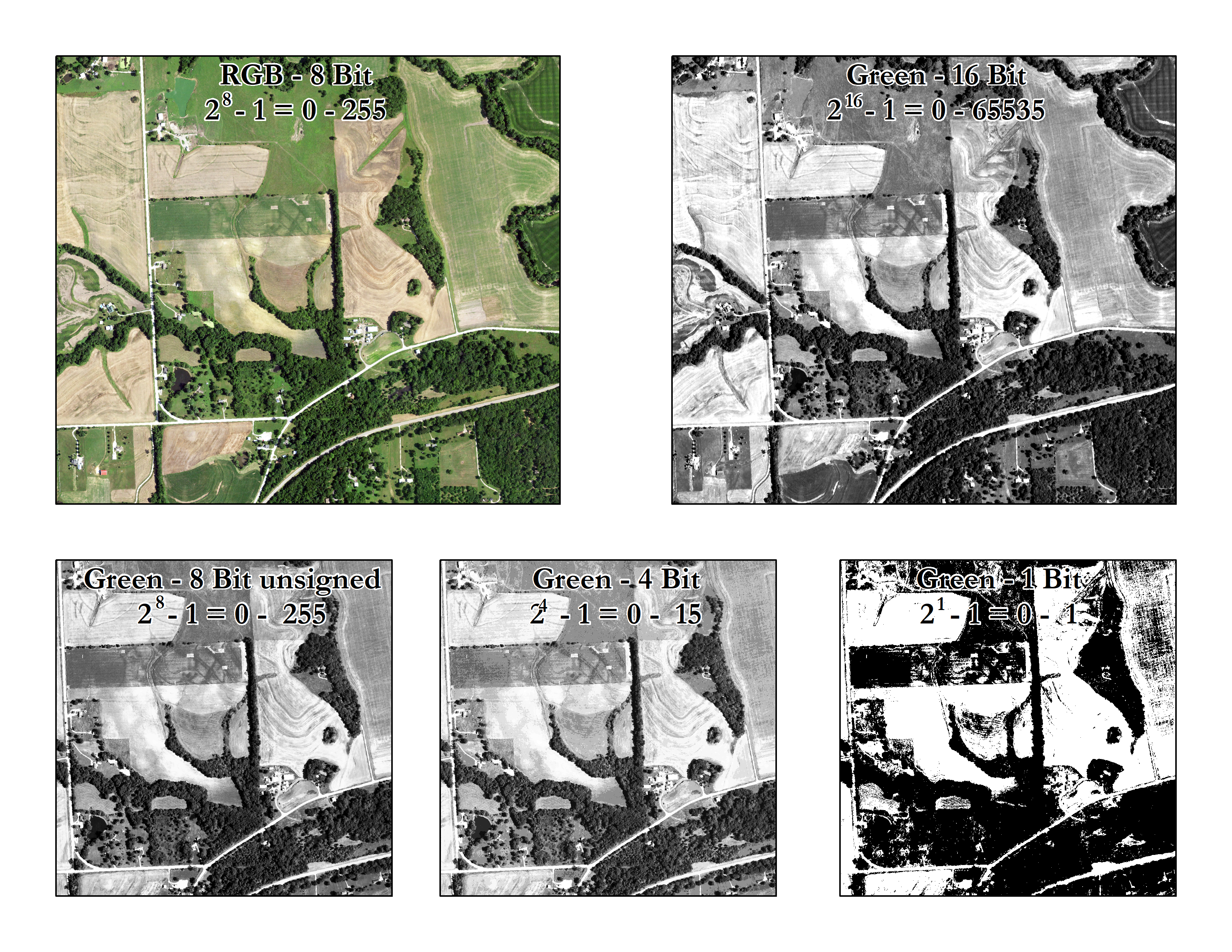
Radiometric resolution: Radiometric resolution is the number of brightness levels that can be detected by the sensor, also known as radiometric sensitivity, quantization, or simply the number of bits per pixel.
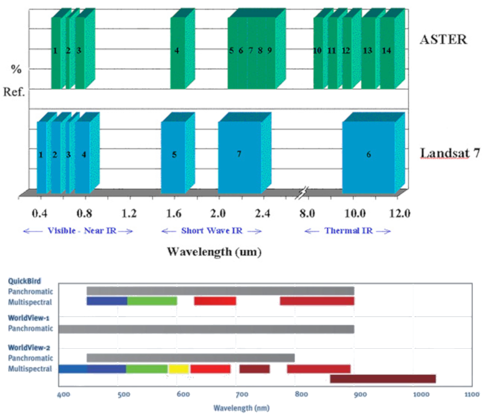
Spectral resolution: Spectral resolution refers to the number and position of the sensor bands along the EM spectrum.
Spatial resolution: Spatial resolution is the ground distance of the pixel, and is typically reported in meters at nadir at the equator.
Temporal resolution: Temporal resolution, or more directly refereed to as revisit time, is, as the name suggests, the time between a repeated observation of the same place on the globe. Temporal resolution is the result of a number of factors, but the two largest are the swath width and the orbit.
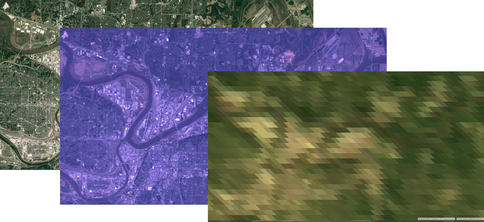
Swath width is the width of a single image, and can either be small or large, The image below (gratefully pilfered from Figure 1 in https://doi-org.www2.lib.ku.edu/10.1016/j.rse.2019.111254) shows the swath of a Landsat-8 OLI orbit (185 km wide, left) compared and a Sentinel-2A MSI orbit (290 km wide, right).
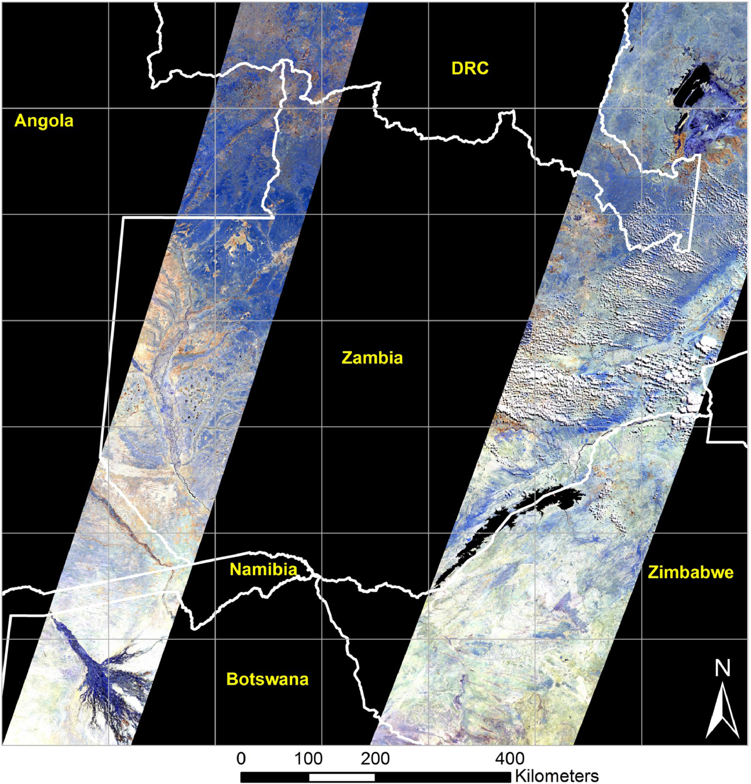
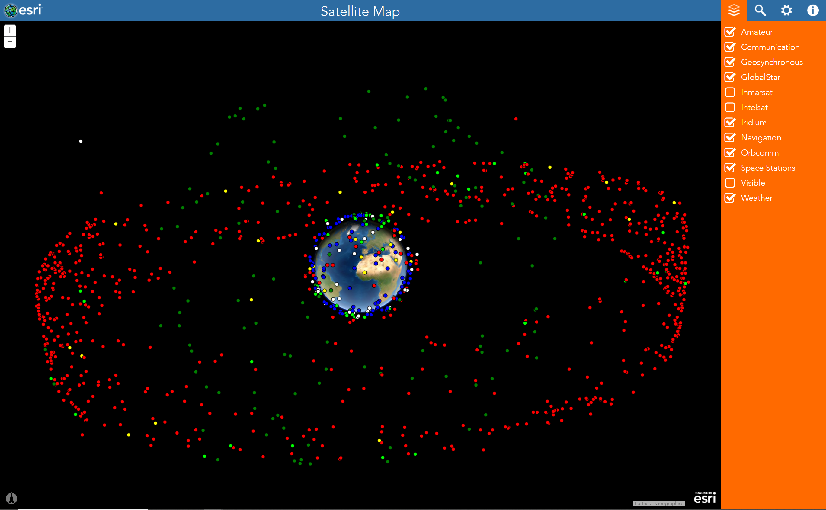
Orbit refers to the direction and nature of the travel path of satellites around a body. There are a number of common orbital patterns satellites exhibit. For more information, see an example of the different orbits and satellites, and explore satellite orbits at this ESRI site.
- Geostationary: The orbit of the sensor is such that it rotates at a speed which maintains the satellites position over the same spot on the earth. Most commonly seen with communication and weather satellites.
- Sun synchronous: The orbit of this satellite follows the sun.
As you might have guessed by now, a proper understanding of remote sensing hinges on a thorough understanding of the data structure and lineage. The Google Earth Engine Dataset catalog has an excellent overview of platforms and datasets avalible for end users, but here we’ll introduce two of my favorite platforms, MODIS, and Landsat
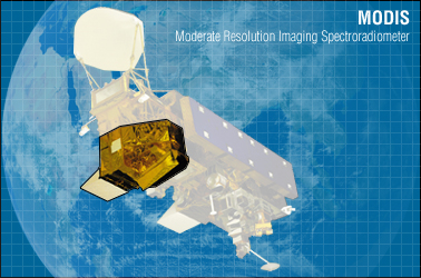 MODIS,(Moderate Resolution Imaging Spectroradiometer) is a key instrument aboard the Terra (originally known as EOS AM-1) and Aqua (originally known as EOS PM-1) satellites. These are passive remote sensing platforms, and so follow a sun synchronous orbit. Terra’s orbit around the Earth is timed so that it passes from north to south across the equator in the morning, while Aqua passes south to north over the equator in the afternoon. Terra MODIS and Aqua MODIS are viewing the entire Earth’s surface every 1 to 2 days, acquiring data in 36 spectral bands.
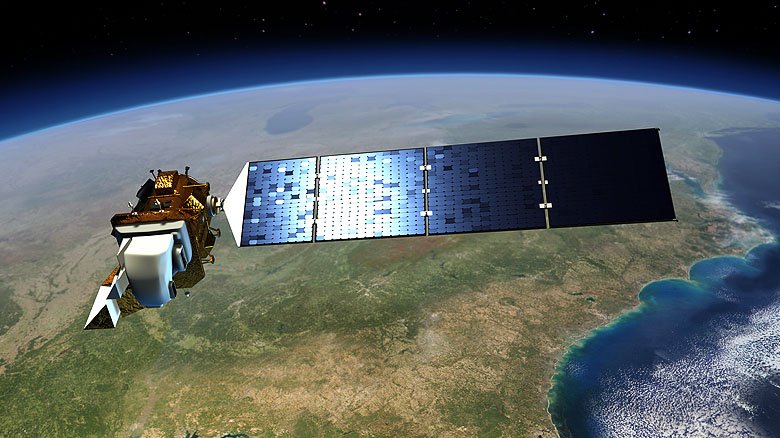 The Landsat program is the longest-running enterprise for acquisition of satellite imagery of Earth. It is a joint NASA/USGS program. Back in July of 1972, the first satellite was launched, and eventually became known as Landsat 1. The most recent satellite, Landsat 8, was launched on February 11, 2013, and is still currently operational. There are a few different sensors onboard, which are outlined below. Landsat 1 through 5 carried the Landsat Multispectral Scanner (MSS). Landsat 4 and 5 carried both the MSS and Thematic Mapper (TM) instruments. Landsat 7 uses the Enhanced Thematic Mapper Plus (ETM+) scanner. Landsat 8 uses two instruments, the Operational Land Imager (OLI) for optical bands and the Thermal Infrared Sensor (TIRS) for thermal bands. Handy charts for these instruments can be found on the wikipedia page.
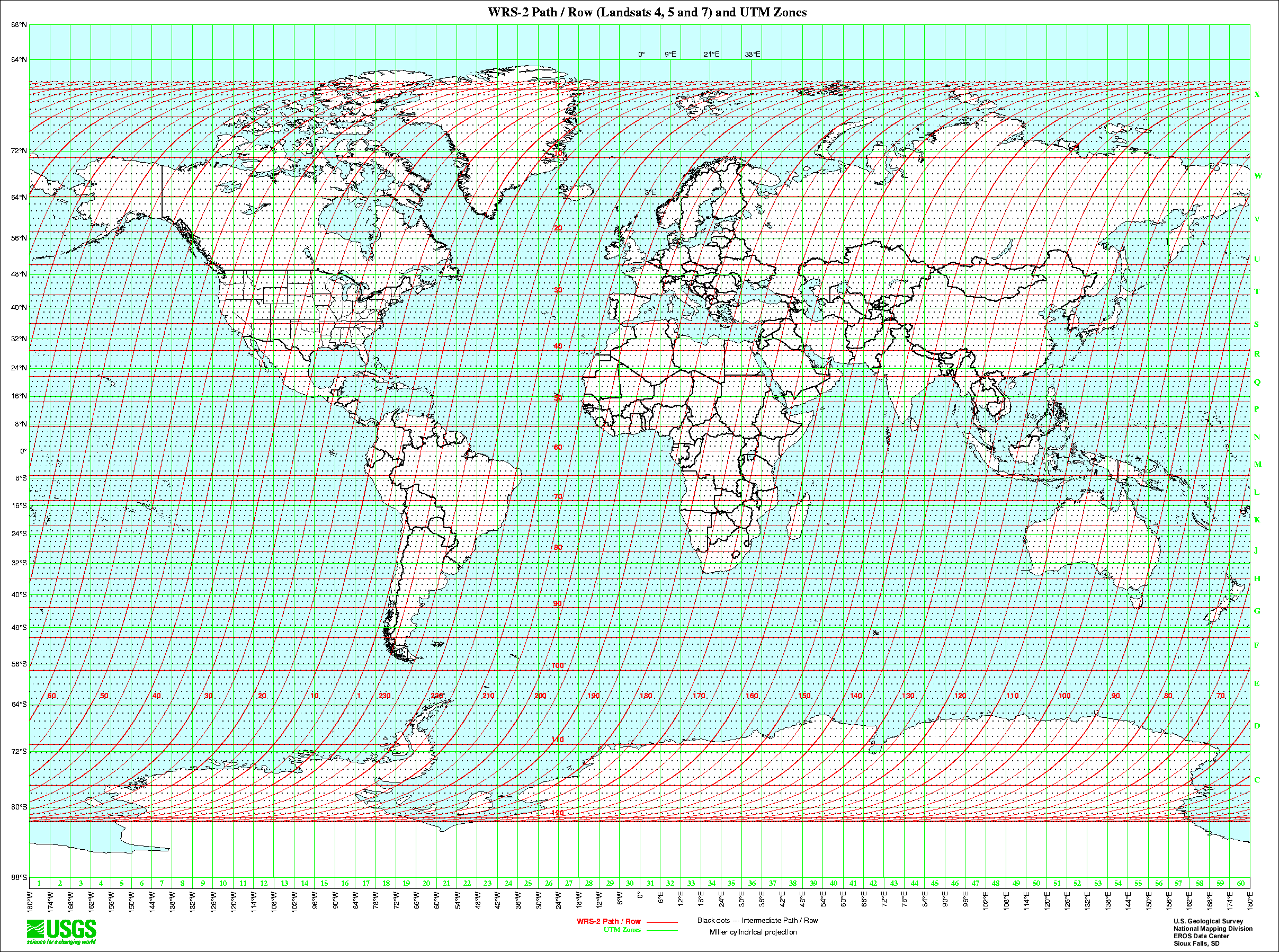
Landsat is distributed in tiles (called scenes) that are identified by their path and row. Although these designations are somewhat arbitrary (in that they provide little geographic context, what does path 34 row 58 tell you?), they are a consistent means of identifying and disseminating tiles.
 https://www.usgs.gov/land-resources/nli/landsat/landsat-shapefiles-and-kml-files
With so much data being collected, you can imagine that a naming convention can get pretty convoluted, and if you don’t work with this data commonly, you’ll need to look up this information each time you need it. However, it’s worthwhile to introduce it here. Landsat collection 1 Level-1 products are all identified using the following naming convention.
LXSS_LLLL_PPPRRR_YYYYMMDD_yyyymmdd_CC_TX
Where:
L = Landsat X = Sensor (“C”=OLI/TIRS combined, “O”=OLI-only, “T”=TIRS-only, “E”=ETM+, “T”=“TM, “M”=MSS) SS = Satellite (”07”=Landsat 7, “08”=Landsat 8) LLL = Processing correction level (L1TP/L1GT/L1GS) PPP = WRS path RRR = WRS row YYYYMMDD = Acquisition year, month, day yyyymmdd - Processing year, month, day CC = Collection number (01, 02, …) TX = Collection category (“RT”=Real-Time, “T1”=Tier 1, “T2”=Tier 2)
Example: LC08_L1GT_029030_20151209_20160131_01_RT Means: Landsat 8; OLI/TIRS combined; processing correction level L1GT; path 029; row 030; acquired December 9, 2015; processed January 31, 2016; Collection 1; Real-Time
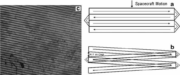
There are quirks to every remote sensing product, but landsat 7 has one of the most unique. Unlike other platforms, such as the Hubble space telescope, these remote sensing platforms do not have the benefit of maintenance after being placed in orbit. So, in June of 2003, when the landsat 7 scan line corrector (slc) module failed, data from half of the collected data was no longer viable. This scan line correcter is responsible for adjusting the position of the sensor as it scanned the earth. The result is a charicteristic striping of the data. There have been numerous efforts to correct for this failure, but for now, just know that most landsat 7 data will look rather zebra-esque.
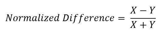
There are a number of uses for remote sensing data, but one of the cornerstones of remote sensing is the normalized difference index. If we take two numbers and subtract them, and divide that by the sum of those same two numbers, we end up with a number that can range from -1 to 1. This normalization can tell us a lot about a process, and is performed for a wide variety of earth classification operations such as snow (NDSI), water (NDWI), and vegetative health (NDVI).
The latter, NDVI, is an often performed analysis to give us a roughly quantitative analysis of the vegetative health of a system. When sunlight strikes objects, some wavelengths of this spectrum are absorbed and other wavelengths are reflected. The pigment in plant leaves, chlorophyll, strongly absorbs visible light (from 0.4 to 0.7 µm) for use in photosynthesis, whereas the cell structure of the leaves strongly reflects near-infrared light (from 0.7 to 1.1 µm). The more leaves a plant has, the more these wavelengths of light are affected. NDVI values are fairly relative (the difference between 0.5 to 0.6 is not generally quantifiable), but in general, anything above 0.2 is vegetation, and higher values are roughly equivalent to more vegetation.
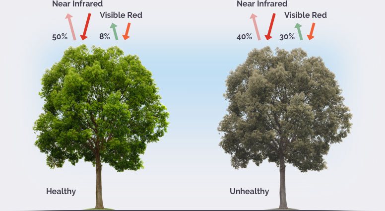
Image from https://eos.com/ndvi/
Let’s use our newfound knowledge to perform one of the most common operations one might want to take, a change detection study. Let’s explore how NDVI changes by land cover type between summer and fall. We’ll use landsat 8. If we look back at the landsat 8 OLS sensor (copied below), we can see that those wavelengths are equivalent to bands 4 and 5.
| Band number | Spectral resolution | Spatial Resolution |
|---|---|---|
| Band 1 | Visible (0.43 - 0.45 µm) | 30 m |
| Band 2 | Visible (0.450 - 0.51 µm) | 30 m |
| Band 3 | Visible (0.53 - 0.59 µm) | 30 m |
| Band 4 | Red (0.64 - 0.67 µm) | 30 m |
| Band 5 | Near-Infrared (0.85 - 0.88 µm) | 30 m |
| Band 6 | SWIR 1(1.57 - 1.65 µm) | 30 m |
| Band 7 | SWIR 2 (2.11 - 2.29 µm) | 30 m |
| Band 8 | Panchromatic (PAN) (0.50 - 0.68 µm) | 15 m |
| Band 9 | Near-Infrared (0.85 - 0.88 µm) | 30 m |
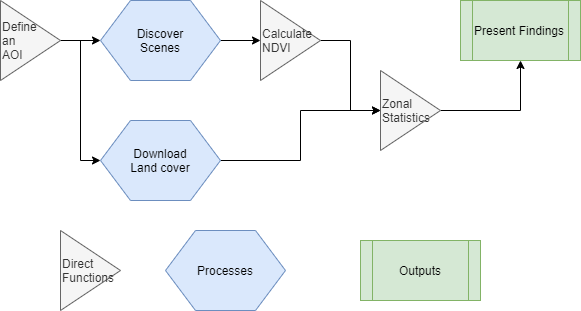
Let’s lay out our workflow conceptually. We’ll first establish an area over which we’ll perform the analysis. Next, we’ll scrape an amazon web service to identify suitable data to use for our analysis, and grab land cover data to perform our analysis. Afterwards, we’ll calculate NDVI and perform our zonal statistics using our land cover. Finally, we’ll create a pretty image as our output image.
You may notice a slightly unique naming convention in the code:
# Pick an AOI
xx <- list()
xx$AOI_center...
I like to create an empty list and stuff all cartographic variables into a single place for easy access when it comes time to create outputs. This also makes it easer to create web apps (the global file then only has to return the list), but that will be a topic for a later date.
# Last build: 7/30/20
# install.packages("devtools")  # Will throw errors if RTools is not installed, you can ignore this for the remained of installation
# install.packages("geosphere")  # For geodesic buffer function
# install.packages("leaflet")  # For visualization
# install.packages("leafem")  # For visualization
# install.packages("raster") # for raster vis
# library(devtools, quietly = TRUE)
# devtools::install_github("ropensci/FedData")  # For easy NLCD download
# devtools::install_github(c("ropensci/getlandsat"))  # For easy landsat download

library(raster, quietly = TRUE)  # vis
library(dplyr, quietly = TRUE)  # Syntax sugar
library(lubridate, quietly = TRUE)  # more syntax sugar
library(rgeos, quietly = TRUE)  # second buffer function
library(jsonlite, quietly = TRUE)  # API query
library(httr, quietly = TRUE)  # web download
library(leaflet, quietly = TRUE)  # vis
library(leafem, quietly = TRUE)  # vis
library(htmltools, quietly = TRUE)  # vis
library(FedData, quietly = TRUE)  # Easy NLCD
library(getlandsat, quietly = TRUE)  # Easy landsat
We’ll use a few helper functions to help us accomplish this task, one to plot a point in the world for use as the centroid of our AOI, and another to generate the approprite utm epsg for that point.
## Helper functions

## geocoding function using OSM Nominatim API -- details: http://wiki.openstreetmap.org/wiki/Nominatim
## Inputs: a human readable address or colloquial name string
## Outputs: success: a sf point with lat and long | Failure: an empty dataframe
## modified from: D.Kisler @ https://datascienceplus.com/osm-nominatim-with-r-getting-locations-geo-coordinates-by-its-address/
nominatim_osm <- function(address = NULL) {
  # Construct a url request
  d <- jsonlite::fromJSON(
    gsub('\\@addr\\@', gsub('\\s+', '\\%20', address), 'http://nominatim.openstreetmap.org/search/@addr@?format=json&addressdetails=0&limit=1'))

  # return parsed sf point
  return(
    sf::st_as_sf(d %>% select('lon','lat','display_name'),
                 coords=c("lon","lat"),
                 crs=sf::st_crs(4326),
                 remove=TRUE)
  )
}

## geodesic buffer function -- details: http://wiki.openstreetmap.org/wiki/Nominatim
## Inputs: a coordinate pair in EPSG:4326
## Outputs: the equivelent UTM zone EPSG
## all credit to Robin Lovelace, Jakub Nowosad, Jannes Muenchow @ https://geocompr.robinlovelace.net/reproj-geo-data.html
lonlat2UTM = function(lonlat) {
  utm = (floor((lonlat[1] + 180) / 6) %% 60) + 1
  if(lonlat[2] > 0) {
    utm + 32600
  } else{
    utm + 32700
  }
}
First, let’s define our AOI and a small buffer
# set a working directory
setwd("C:/Users/Cornholio/Desktop/coolclass") # your own filepath here

# Pick an AOI and (small) buffer distance
xx <- list()
xx$AOI_center <- nominatim_osm("Lawrence, KS")
# xx$AOI_center <- sp::SpatialPoints(list(-95.23595,38.97194)) %>% sf::st_as_sfc() %>% sf::st_set_crs(4326) # or spesify a lon/lat point
mybufferdist_m = 1200

# Buffer AOI point
# get UTM epsg
aoiUTMEPSG <- lonlat2UTM(sf::st_coordinates(xx$AOI_center))
# reproject
xx$AOI_center_utm <- sf::st_transform(xx$AOI_center,aoiUTMEPSG)
# buffer (gBuffer requires a spatial object, not an sf), return to sf, reattach crs
xx$AOI_buffer_utm <- rgeos::gBuffer(sp::SpatialPoints(sf::st_coordinates(xx$AOI_center_utm)),width = mybufferdist_m) %>%
  sf::st_as_sfc() %>%
  sf::st_set_crs(aoiUTMEPSG)

xx$AOI_buffer_utm <- rgeos::gBuffer(sp::SpatialPoints(sf::st_coordinates(xx$AOI_center_utm)),width = mybufferdist_m) %>%
  sf::st_as_sfc()
sf::st_crs(xx$AOI_buffer_utm) = aoiUTMEPSG

xx$AOI_buffer <- sf::st_transform(xx$AOI_buffer_utm, 4326) # reproject back to wgs84
xx$processbounds <- sf::st_bbox(xx$AOI_buffer)
# st_bbox doesn't return a spatial object, so we'll correct for that here
xx$AOI_bbox <- sf::st_bbox(xx$AOI_buffer) %>% sf::st_as_sfc() %>% sf::st_set_crs(4326)

# Finally, let's make sure everything plots as expected
leaflet() %>%
  addProviderTiles(providers$Stamen.TonerLite, group = "Base Map") %>%
  addPolygons(data=xx$AOI_buffer,color="red")
# Aside: was geodesic buffering necessary?  Let's test using a "relative" simplification!
# @ https://planetcalc.com/7721/  --  WGS 84 defines ellipsoid parameters as:
a = 6378137.0        # Semi-major axis in meters
b = 6356752.314245   # Semi-minor axis in meters
l = sf::st_coordinates(xx$AOI_center)[2]
radius_globe_meters <-
  sqrt((((((a^2)*cos(l))^2)+(((b^2)*sin(l))^2)))/((((a*cos(l))^2)+((b*sin(l))^2))))
radius_degrees <- mybufferdist_m/radius_globe_meters
# xx$AOI_badbuffer <- rgeos::gBuffer(sp::SpatialPoints(sf::st_coordinates(xx$AOI_center)),width = radius_degrees) %>%
#   sf::st_as_sfc() %>%
#   sf::st_set_crs(4326)

# all credit to https://geocompr.robinlovelace.net/reproj-geo-data.html
lonlat2UTM = function(lonlat) {
  utm = (floor((lonlat[1] + 180) / 6) %% 60) + 1
  if(lonlat[2] > 0) {
    utm + 32600
  } else{
    utm + 32700
  }
}
aoiUTMEPSG <- lonlat2UTM(sf::st_coordinates(xx$AOI_center))
xx$AOI_center_utm <- sf::st_transform(xx$AOI_center,newEPSG)

xx$AOI_badbuffer <- rgeos::gBuffer(sp::SpatialPoints(sf::st_coordinates(xx$AOI_center_utm)),width = mybufferdist_m) %>%
  sf::st_as_sfc() %>%
  sf::st_set_crs(aoiUTMEPSG)
xx$AOI_badbuffer <- sf::st_transform(xx$AOI_badbuffer,4326)

# and check visually
leaflet() %>%
  addProviderTiles(providers$Stamen.TonerLite, group = "Base Map") %>%
  addPolygons(data=xx$AOI_buffer,color="red") %>%
  addPolygons(data=xx$AOI_badbuffer,color="green")
# Conclusion: it's too late for me to be futzing around with this....  Any ideas?
We next need to identify scenes for use. Landsat distriburts scenes by path and row more here
# discover path and row
httr::GET('https://prd-wret.s3.us-west-2.amazonaws.com/assets/palladium/production/s3fs-public/atoms/files/WRS2_descending_0.zip',
          write_disk(paste0(getwd(), "/WRS2_descending_0.zip")))
unzip(paste0(getwd(), "/WRS2_descending_0.zip"), exdir = getwd())
xx$pathrow <- sf::read_sf(paste0(getwd(), "/WRS2_descending.shp"))

# That pathrow file covers the entire globe, let's make this a tiny bit gentler to visualize
# and subset that to just the pathrows that intersect our AOI
xx$pathrow_subset <- xx$pathrow[xx$AOI_bbox,]

# explore geographic context
leaflet() %>%
  addProviderTiles(providers$Stamen.TonerLite, group = "Base Map") %>%
  addPolygons(data=xx$AOI_buffer,color="red") %>%
  addPolygons(data=xx$pathrow_subset,
              color="black",
              fill = FALSE,
              label = mapply(function(x, y) {
                HTML(sprintf("<em>Path/row:</em>%s-%s", htmlEscape(x), htmlEscape(y)))},
                xx$pathrow_subset$PATH, xx$pathrow_subset$ROW, SIMPLIFY = F),
              labelOptions = lapply(1:nrow(xx$pathrow_subset), function(x) {
                labelOptions(noHide = T)
              })) %>%
  fitBounds(as.numeric(floor(xx$processbounds$xmin)),
            as.numeric(floor(xx$processbounds$ymin)),
            as.numeric(ceiling(xx$processbounds$xmax)),
            as.numeric(ceiling(xx$processbounds$ymax)))
That visualization was perhaps a bit overkill, all we needed to do here is ensure that our AOI is completely enclosed within a single path/row. We’ll cover mosaicking (stitching together multiple scenes at once) later in the course, but for now if you end up inside more than one, adjust your point until you fall squarely within a single tile (or entirely in a crossover section).
Having identified our path and row, let’s now explore the landsat catalog
# Find the scenes for your path and row
summerdaterange <- interval(as.POSIXct("2015-06-01 00:00:00"),
                            as.POSIXct("2015-09-01 00:00:00"))

summerscene <- getlandsat::lsat_scenes() %>%
  filter(row == xx$pathrow_subset$ROW) %>%                # Filter for row...
  filter(path == xx$pathrow_subset$PATH) %>%              # and path
  filter(acquisitionDate %within% summerdaterange) %>%    # get our date
  arrange(cloudCover) %>%                                 # put the least cloudy scene first
  .[1,]                                                   # and peel it off

summerscene
# as we see, there is a suitable cloud free scene, let's look at it's formatting:


# In addition to making a handy scene scrapper, the getLandsat package is also a wrapper to download scenes by name
summer_band4_path <- getlandsat::lsat_image(paste0(summerscene$entityId,"_B4.TIF"))
summer_band4 <- raster::raster(summer_band4_path)
xx$summer_band4 <- raster::mask(summer_band4,sf::as_Spatial(xx$AOI_buffer_utm))

# and visualize
leaflet() %>%
  addProviderTiles(providers$Stamen.TonerLite, group = "Base Map") %>%
  addRasterImage(xx$summer_band4, layerId = "values") %>%
  addMouseCoordinates() %>%
  addImageQuery(xx$summer_band4, type="mousemove", layerId = "values")

# Lets do the same for band 5
summer_band5_path <- getlandsat::lsat_image(paste0(summerscene$entityId,"_B5.TIF"))
summer_band5 <- raster::raster(summer_band5_path)
xx$summer_band5 <- raster::mask(summer_band5,sf::as_Spatial(xx$AOI_buffer_utm))
Now, let’s perform our local operation
summer_ndvi <- raster::overlay(xx$summer_band5, xx$summer_band4, fun = function(r1, r2) { return( (r1 - r2)/(r1 + r2)) })

# and visualize
leaflet() %>%
  addProviderTiles(providers$Stamen.TonerLite, group = "Base Map") %>%
  addRasterImage(summer_ndvi, layerId = "values") %>%
  addMouseCoordinates() %>%
  addImageQuery(summer_ndvi, type="mousemove", layerId = "values")
Now that we have NDVI, we need a land cover dataset. more here about NLCD
NLCD <- FedData::get_nlcd(template = sf::as_Spatial(xx$AOI_buffer_utm),
                          year = 2016,
                          dataset = "Land_Cover",
                          label = "AOI")
# --------------------------------------------------------------------------------------------
# backup, because MRLC service is down more often than it's up...
# this may take a while because we're grabbing all of CONUS
httr::GET('https://s3-us-west-2.amazonaws.com/mrlc/NLCD_2016_Land_Cover_L48_20190424.zip',
          write_disk(paste0(getwd(), "/NLCD_2016_Land_Cover_L48.zip")))
unzip(paste0(getwd(), "/NLCD_2016_Land_Cover_L48.zip"), exdir = getwd())
NLCD <- raster::raster(paste0(getwd(),'/NLCD_2016_Land_Cover_L48_20190424.img'))
# --------------------------------------------------------------------------------------------
landcover_utm <- NLCD %>%
  raster::projectRaster(crs = raster::crs(xx$summer_band4)) %>%
  raster::mask(sf::as_Spatial(xx$AOI_buffer_utm))

landcover_utm <- NLCD %>%
  raster::projectRaster(crs = raster::crs(xx$summer_band4)) %>%
  raster::mask(sf::as_Spatial(xx$AOI_buffer_utm))
# Finally, we'll (visualize) write the raster to disk, garbage collect, and reload the layer as that was a fairly
# expensive set of computations we just performed
# Land cover color pallete values
xx$NLCD.pal <- c("#5475A8","#FFFFFF","#E8D1D1","#E29E8C","#FF0000","#B50000","#D2CDC0","#85C77E","#38814E","#D4E7B0","#AF963C","#DCCA8F","#FDE9AA","#D1D182","#A3CC51","#82BA9E","#FBF65D","#CA9146","#C8E6F8","#64B3D5")
xx$NLCD.val <- as.numeric(c(11,12,21,22,23,24,31,41,42,43,51,52,71,72,73,74,81,82,90,95))
xx$NLCD.text <- c("Open Water","Perennial Ice/Snow","Developed, Open Space","Developed, Low Intensity","Developed, Medium Intensity","Developed, High Intensity","Barren Land","Deciduous Forest","Evergreen Forest","Mixed Forest",
                  "Dwarf Scrub","Shrub/Scrub","Grassland/Herbaceous","Sedge/Herbaceous","Lichens","Moss","Pasture/Hay","Cultivated Crops","Woody Wetlands","Emergent Herbaceous Wetlands")
xx$NLCD.vis <- colorFactor(palette = xx$NLCD.pal,
                           domain = xx$NLCD.val)

leaflet() %>%
  addProviderTiles(providers$Stamen.TonerLite, group = "Base Map") %>%
  addRasterImage(NLCD,colors=xx$NLCD.vis) %>%
  addLegend("bottomright",
            title = "National Land Cover Data",
            colors = xx$NLCD.pal,
            labels = xx$NLCD.text)

raster::writeRaster(landcover_utm,paste0(getwd(),"/AOI_LC.tif"))
gc()
xx$landcover <- raster::raster(paste0(getwd(),"/AOI_LC.tif"))
We now have all the pieces we need to generate the desired statistics, our last step is to perform the zonal statistics
xx$summer_ndvi <- raster::resample(summer_ndvi,xx$landcover,method="bilinear")
xx$zonalstats <- raster::zonal(xx$summer_ndvi, xx$landcover, fun='mean', digits=0, na.rm=TRUE)
add here https://developers.google.com/earth-engine/datasets/catalog/LANDSAT_LC08_C01_T1_32DAY_NDVI